1.6: Time-Harmonic Solutions of the Wave Equation

The fact that, in the frequently occurring circumstance in which light interacts with a homogeneous dielectric, all components of the electromagnetic field satisfy the scalar wave equation, justifies the study of solutions of this equation. Since in most cases in optics monochromatic fields are considered, we will focus our attention on time-harmonic solutions of the wave equation.

1.5.1 Time-Harmonic Plane Waves

Time-harmonic solutions depend on time by a cosine or a sine. One can easily verify by substitution that

\[U(r,t)=Acos(kx-ωt+ϕ), \nonumber \]

where A > 0 and ϕ are constants, is a solution of (1.4.10), provided that

\[k = ω(Eµ_{0})^{1/2} = ωn(E_{0}µ_{0})^{1/2} = nk_{0}, \nonumber \]

where k₀ = ω(E₀µ₀)^1/2 is the wave number in vacuum. The frequency ω > 0 can be chosen arbitrarily. The wave number k in the material is then determined by (\(\PageIndex{2}\)). We define T = 2π/ω and λ = 2π/k as the period and the wavelength in the material, respectively. Furthermore, λ₀ = 2π/k₀ is the wavelength in vacuum.

Remark. When we speak of "the wavelength", we always mean the wavelength in vacuum.

We can write (\(\PageIndex{1}\)) in the form

\[U(x,t)=Acos[k(x-\dfrac{c}{n}t)+ϕ], \nonumber \]

where c/n = 1/(Eµ₀)^1/2 is the speed of light in the material. A is the amplitude and the argument under the cosine: k(x-ct/n)+ϕ is called the phase at position x and at time t. A wavefront is a set of space-time points where the phase is constant:

\[x-\dfrac{c}{n}t=constant. \nonumber \]

At any fixed time t the wave fronts are planes (in this case perpendicular to the x-axis), and therefore the wave is called a plane wave. As time proceeds, the wavefronts move with velocity c/n in the positive x-direction.

A time-harmonic plane wave propagating in an arbitrary direction is given by

\[U(r,t)=Acos(k · r-ωt+ϕ), \nonumber \]

where A and ϕ are again constants and k = k_xx + k_yy + k_zz is the wave vector. The wavefronts are given by the set of all space-time points (r, t) for which the phase k · r − ωt + ϕ is constant, i.e. for which

\[k · r − ωt = constant. \nonumber \]

At fixed times the wavefronts are planes perpendicular to the direction of k as shown in Fig.\(\PageIndex{1}\) Eq. (\(\PageIndex{5}\)) is a solution of (1.4.10) provided that

\[k_{x}^2+k_{y}^2+k_{z}^2=ω^2Eµ_{0}=ω^2n^2E_{0}µ_{0}=k_{0}^2n^2. \nonumber \]

The direction of the wave vector can be chosen arbitrarily, but its length is determined by the frequency ω.

1.5.2 Complex Notation for Time-Harmonic Functions

We consider a general time-harmonic solution of the wave equation (1.4.8):

\[U(r, t) = A(r) cos(ϕ(r) − ωt), \nonumber \]

where the amplitude A(r) > 0 and the phase ϕ(r) are functions of position r. The wavefronts consist of space-time points (r, t) where the phase is constant:

\[ϕ(r) − ωt = constant. \nonumber \]

At fixed time t, the sets of constant phase: ϕ(r) = ωt + constant are surfaces which in general are not planes, hence the solution in general is not a plane wave. Eq. (\(\PageIndex{9}\)) could for example be a wave with spherical wavefronts, as discussed below.

Remark. A plane wave is infinitely extended and carries and transports an infinite amount of electromagnetic energy. A plane plane can therefore not exist in reality, but it is nevertheless a usual idealisation because, as will be demonstrated in in Section 7.1, every time-harmonic solution of the wave equation can always be expanded in terms of plane waves of the form (\(\PageIndex{5}\)).

For time-harmonic solutions it is often convenient to use complex notation. Define the complex amplitude by:

\[U(r) = A(r)e^{iϕ(r)} \nonumber \]

Figure \(\PageIndex{1}\): Planes of constant phase.

i.e. the modulus of the complex number U(r) is the amplitude A(r) and the argument of U(r) is the phase ϕ(r) at t = 0. The time-dependent part of the phase: −ωt is thus separated from the space-dependent part of the phase. Then (\(\PageIndex{8}\)) can be written as

\[U(r, t) = Re [ U(r)e^{−iωt}] . \nonumber \]

Hence U(r, t) is the real part of the complex time-harmonic function

\[U(r)e^{−iωt} . \nonumber \]

Remark. The complex amplitude U(r) is also called the complex field. In the case of vector fields such as E and H we speak of complex vector fields, or simply complex fields. Complex amplitudes and complex (vector) fields are only functions of position r; the time dependent factor exp(−iωt) is omitted. To get the physical meaningful real quantity, the complex amplitude or complex field first has to be multiplied by exp(−iωt) and then the real part must be taken.

The following convention is used throughout this book:

Real-valued physical quantities (whether they are time-harmonic or have more general time dependence) are denoted by a calligraphic letter, e.g. U, ε_x, or H_x. The symbols are bold when we are dealing with a vector, e.g. ε or H. The complex amplitude of a time-harmonic function is linked to the real physical quantity by (\(\PageIndex{11}\)) and is written as an ordinary letter such as U and E.

It is easier to calculate with complex amplitudes (complex fields) than with trigonometric functions (cosine and sine). As long as all the operations carried out on the functions are linear, the operations can be carried out on the complex quantities. To get the real-valued physical quantity of the result (i.e. the physical meaningful result), multiply the finally obtained complex amplitude by exp(−iωt) and take the real part. The reason that this works is that taking the real part commutes with linear operations, i.e. taking first the real part to get the real-valued physical quantity and then operating on this real physical quantity gives the same result as operating on the complex scalar and taking the real part at the end.

By substituting (\(\PageIndex{12}\)) into the wave equation (1.4.10) we get

\[\bigtriangledown^2U(r,t)-n^2E_{0}µ_{0}\dfrac{\partial^2{U(r,t)}}{\partial{t^2}}=Re[\bigtriangledown^2U(r)e^{−iωt}]-n^2E_{0}µ_{0}Re[U(r)\dfrac{\partial^2{e^{-iωt}}}{\partial^2}]=Re[\bigtriangledown^2U(r)+ω^2n^2E_{0}µ_{0}U(r)]e^{-iωt}. \nonumber \]

Since this must vanish for all times t, it follows that the complex expression between the brackets {.} must vanish. To see this, consider for example the two instances t = 0 and t = π/(2ω. Hence we conclude that the complex amplitude satisfies

\[\bigtriangledown^2U(r)+k_{0}^2n^2U(r)=0, Helmholtz\space Equation, \nonumber \]

where k₀ = ω(E₀µ₀)^1/2 is the wave number in vacuum.

Remark. The complex quantity of which the real part has to be taken is: U exp(−iωt). It is not necessary to drag the time-dependent factor exp(−iωt) along in the computations: it suffices to calculate only with the complex amplitude U, then multiply by exp(−iωt) and then take the real part. However, when a derivative with respect to time is to be taken: ∂/∂t the complex field much be multiplied by −iω. This is also done in the time-harmonic Maxwell’s equations in Section 1.6 below.

1.5.3 Time-Harmonic Spherical Waves

A spherical wave depends on position only by the distance to a fixed point. For simplicity we choose the origin of our coordinate system at this point. We thus seek a solution of the form U(r, t) with r = ( x2 + y2 + z2)1/2. For spherical symmetric functions we have

\[\bigtriangledown^2U(r,t)=\dfrac{1}{r}\dfrac{\partial^2}{\partial{r^2}}[rU(r,t)] \nonumber \]

It is easy to see that outside of the origin

\[U(r,t)=\dfrac{f(±r-ct/n)}{r}, \nonumber \]

satisfies (1.47) for any choice for the function f, where, as before, c = 1/(E0µ0)1/2 is the speed of light and n = (E/E0)1/2. Of particular interest are time-harmonic spherical waves:

\[U(r, t) = \dfrac{A}{r}cos[ k ( ±r − \dfrac{c}{n}t) + ϕ] = \dfrac{A}{r}cos(±kr − ωt + ϕ) \nonumber \]

where A is a constant

\[k = nω/c. \nonumber \]

and ±kr − ωt + ϕ is the phase at r and at time t. The wavefronts are space-time points (r, t) where the phase is constant:

\[±kr − ωt = constant, \nonumber \]

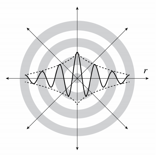
which are spheres which move with the speed of light in the radial direction. When the + sign is chosen, the wave propagates outwards, i.e. away from the origin. The wave is then radiated by a source at the origin. Indeed, if the + sign holds in (\(\PageIndex{17}\)), then if time t increases, (\(\PageIndex{19}\)) implies that a surface of constant phase moves outwards. Similarly, if the − sign holds, the wave propagates towards the origin which then acts as a sink. The amplitude of the wave A/r is proportional to the inverse distance to the source of sink. Since the local flux of energy is proportional to the square A²/r² , the total flux through the surface of any sphere with centre the origin is independent of the radius of the sphere. Since there is a source or a sink at the origin, (\(\PageIndex{17}\)) satisfies (\(\PageIndex{15}\)) only outside of the origin. There is a δ-function as source density on the right-hand side:

\[Eμ_{0}\dfrac{\partial^2}{\partial{t^2}}U(r, t) − \bigtriangledown^2U(r, t) = 4πA δ(r), \nonumber \]

where the right-hand side corresponds to either a source or sink at the origin, depending on the sign chosen in the phase.

Figure \(\PageIndex{2}\): Spherical wavefronts with amplitude decreasing with distance.

Figure \(\PageIndex{3}\): Planes of constant phase in cross-section. For an observer at large distance to the source the spherical wave looks similar to a plane wave.

Using complex notation we have for the outwards propagating wave:

\[U(r, t) = Re [ U(r)e^{−iωt}] = Re[\dfrac{A}{r}e^{i(kr−iωt)}] \nonumber \]

with U(r) = A exp(ikr)/r and A = A exp(iϕ), where ϕ is the argument and A the modulus of the complex number A.

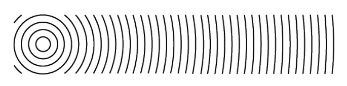
In Figure \(\PageIndex{2}\) and Figure \(\PageIndex{3}\) spherical wavefronts are shown. For an observer who is at a large distance from the source, the spherical wave looks like a plane wave which propagates from the source towards the observer (or in the opposite direction, if there is a sink).