1.7: Time-Harmonic Maxwell Equations in Matter

We now return to the Maxwell equations and consider time-harmonic electromagnetic fields, because these are by far the most important fields in optics. Using complex notation we have

\[E(r, t) = Re [ E(r)e^{−iωt}], \nonumber \]

with E_x(r) = |E_x(r)|e^iϕx(r), E_y(r) = |E_y(r)|e^iϕy(r), E_z(r) = |E_z(r)|e^iϕz(r), where ϕ_x(r) is the argument of the complex number E_x(r) etc. With similar notations for the magnetic field, we obtain by substitution into Maxwell’s equations (1.3.12), (1.3.13), (1.3.14) and (1.3.15), the time-harmonic Maxwell equations for the complex fields:

\[∇ × E = iωµ_{0}H, Faraday’s\space Law \nonumber \]

\[∇ × H = −iωεE + σE + J_{ext}, Maxwell’s\space Law \nonumber \]

\[∇ · ε E = ρ_{ ext}, Gauss’s\space Law \nonumber \]

\[∇ · H = 0, no\space magnetic\space charge \nonumber \]

where the time derivative has been replaced by multiplication of the complex fields by −iω.

In the time-harmonic Maxwell equations, the conductivity is sometimes included in the imaginary part of the permittivity:

\[E= E_{ 0} [ 1 + χ_{e} + i\dfrac{σ}{ω}]. \nonumber \]

Although it is convenient to do this in Maxwell’s Law (\(\PageIndex{3}\)), one should remember that in Gauss’s Law (\(\PageIndex{4}\)), the original permittivity: E = 1 + χ_e should still be used. When there are no external sources: ρ_ext = 0 and the material is homogeneous (i.e. χ_e and σ are independent of position), then (\(\PageIndex{4}\)) is equivalent to

\[∇ · E = 0. \nonumber \]

Hence in this (important) special case, definition (\(\PageIndex{6}\)) for the permittivity can safely be used without the risk of confusion.

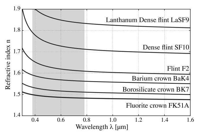
We see that when we use definition (\(\PageIndex{6}\)), the conductivity makes the permittivity complex and depending on frequency. But actually, also for insulators (σ = 0), the permittivity E depends in general on frequency and is complex with a positive imaginary part. The positive imaginary part of E is a measure of the absorption of the light by the material. The property that the permittivity depends on the frequency is called dispersion. Except close to a resonance frequency, the imaginary part of E (ω) is small and the real part is a slowly increasing function of frequency. This is called normal dispersion. This is illustrated with the refractive index of different glass shown in Figure \(\PageIndex{1}\)

Near a resonance, the real part is rapidly changing and decreases with ω (this behaviour is called anomalous dispersion), while the imaginary part has a maximum at the resonance frequency of the material, corresponding to maximum absorption at a resonance as seen in Figure \(\PageIndex{2}\) At optical frequencies, mostly normal dispersion occurs and for small-frequency bands such as in laser light, it is often sufficiently accurate to use the value of the permittivity and the conductivity at the centre frequency of the band.

Figure \(\PageIndex{1}\): Real part n² − κ² and imaginary part 2nκ of the permittivity E = (n + iκ)² , as function of wavelength and of frequency near a resonance.

Figure \(\PageIndex{2}\): Refractive index as function of wavelength for several types of glass (from Wikimedia Commons by Geek3 / CC BY-SA).

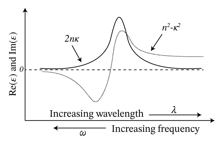
In many books the following notation is used: E = (n + iκ)² , where n and κ ("kappa", not to be confused with the wave number k) are both real and positive, with n the refractive index and κ a measure of the absorption. We then have Re(E ) = n² − κ² and Im(E ) = 2nκ (see Figure \(\PageIndex{1}\)). Note that although n and κ are both positive, Re(E ) can be negative for some frequencies. This happens for metals in the visible part of the spectrum.

Remark. When E depends on frequency, Maxwell’s equations (1.3.13) and (1.3.14) for fields that are not time-harmonic can strictly speaking not be valid, because it is not clear which value of E corresponding to which frequency should be chosen. In fact, in the case of strong dispersion, the products Eε should be replaced by convolutions in the time domain. Since we will almost always consider fields with a narrow-frequency band, we shall not elaborate on this issue further.

1.6.1 Time-Harmonic Electromagnetic Plane Waves

In this section we assume that the material in which the wave propagates has conductivity which vanishes: σ = 0, does not absorb the light and is homogeneous, i.e. that the permittivity E is a real constant. Furthermore, we assume that in the region of space of interest there are no sources. These assumptions imply in particular that (\(\PageIndex{7}\)) holds. The electric field of a time-harmonic plane wave is given by

\[E(r, t) = Re [ E(r)e^{−iωt}], \nonumber \]

with

\[E(r) = Ae^{ik·r}, \nonumber \]

where A is a constant complex vector (i.e. it is independent of position and time):

\[A = A_{x}\hat{x}+ A_{y}\hat{y} + A_{z}\hat{z}, \nonumber \]

with Ax = |Ax|e^iϕx etc.. The wave vector k satisfies (1.5.7). Substitution of (\(\PageIndex{9}\)) into (\(\PageIndex{7}\)) implies that

\[E(r) · k=0 \nonumber \]

for all r and hence (\(\PageIndex{8}\)) implies that also the physical real electric field is in every point r perpendicular to the wave vector: ε(r, t) · k = 0. For simplicity we now choose the wave vector in the direction of the z-axis and we assume that the electric field vector is parallel to the x-axis. This case is called a x-polarised electromagnetic wave. The complex field is then written as

\[E(x)=Ae^{ikz}\hat{x}, \nonumber \]

where k = ω(Eµ₀)^1/2 and A = |A| exp(iϕ). It follows from Faraday’s Law (\(\PageIndex{2}\)) that

\[H(z)=\dfrac{k}{ωµ_{0}}\hat{z}×\hat{x}Ae^{ikz}=(\dfrac{E}{µ_{0}})^{1/2}Ae^{ikz}\hat{y}. \nonumber \]

The real electromagnetic field is thus:

\[ε(z, t) = Re [ E(z)e^{−iωt}] = |A| cos(kz − ωt + ϕ)\hat{x}, \nonumber \]

\[H(z, t) = Re [ H(z)e^{−iωt}] =(\dfrac{E}{µ_{0}})^{1/2}|A| cos(kz − ωt + ϕ)\hat{y}. \nonumber \]

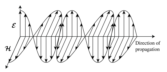
We conclude that in a lossless medium, the electric and magnetic field of a plane wave are in phase and at every point and at every instant perpendicular to the wave vector and to each other. As illustrated in Figure \(\PageIndex{3}\), at any given point both the electric and the magnetic field achieve their maximum and minimum values at the same time.

Figure \(\PageIndex{3}\): The time-harmonic vectors ε and H of a plane polarised wave are perpendicular to each other and to the direction of the wave vector which is also the direction of ε × H.

1.6.2 Field of an Electric Dipole

An other important solution of Maxwell’s equation is the field radiated by a time-harmonic electric dipole, i.e. two opposite charges with equal strength that move time-harmonically around their total centre of mass. In this section the medium is homogeneous, but it may absorb part of the light, i.e. the permittivity may have a nonzero imaginary part. An electric dipole is the classical electromagnetic model for an atom or molecule. Because the optical wavelength is much larger than an atom of molecule, these charges may be considered to be concentrated both in the same point r₀. The charge and current densities of such an elementary dipole are

\[ρ = −p · ∇δ(r − r_{0}), \nonumber \]

\[J = −iωpδ(r − r_{0}), \nonumber \]

with p the dipole vector, defined by

\[p = qa, \nonumber \]

where q > 0 is the positive charge and a is the position vector of the positive with respect to the negative charge.

The field radiated by an electric dipole is very important. It is the fundamental solution of Maxwell’s equations, in the sense that the field radiated by an arbitrary distribution of sources can always be written as a superposition of the fields of elementary electric dipoles. This follows from the fact that Maxwell’s equations are linear and any current distribution can be written as a superposition of elementary dipole currents.

The field radiated by an elementary dipole in r₀ in homogeneous matter can be computed analytically and is given by

\[E(r) = [ k2 \hat{R} × ( p × \hat{R}) + ( 3 \hat{R} · p \hat{R} − p) ( \dfrac{1}{R^2} − \dfrac{ik}{R} )]\dfrac{e^{ikR}}{4πER}, \nonumber \]

\[H(r) =\dfrac{k^2c}{n}(1 +\dfrac{ik}{R})\hat{R} × p\dfrac{e^{ikR}}{4πR}, \nonumber \]

where k = k₀, n = (E/E₀)^1/2, with k₀ the wave number in vacuum and with R = r − r₀. It is seen that the complex electric and magnetic fields are proportional to the complex spherical wave: e^ikR/R discussed in Section 1.5.3, but that these fields contain additional position dependent factors. In particular, at large distance to the dipole:

\[H(r) ≈\dfrac{k^2c}{n}\hat{R} × p\dfrac{e^{ikR}}{4πR}, \nonumber \]

\[E(r) ≈k^2 \hat{R} × (p × \hat{R})\dfrac{e^{ikR}}{4πER}=-(\dfrac{μ_{0}}{E})\hat{R} × H(r).

Figure \(\PageIndex{4}\): Electric and magnetic field lines created by a radiating dipole (from Wikimedia Commons, original JPG due to Averse, SVG by Maschen. / CC0).

In Figure \(\PageIndex{4}\) are drawn the electric and magnetic field lines of a radiating dipole. For an observer at large distance from the dipole, the electric and magnetic fields are perpendicular to each other and perpendicular to the direction of the line of sight R from the dipole to the observer. Furthermore, the electric field is in the plane through the dipole vector p and the vector R, while the magnetic field is perpendicular to this plane. So, for a distant observer the dipole field is similar to that of a plane wave which propagates from the dipole towards the observer and has an electric field parallel to the plane through the dipole and the line of sight R and perpendicular to R. Furthermore, the amplitudes of the electric and magnetic fields depend on the direction of the line of sight, with the field vanishing when the line of sight R is parallel to the dipole vector p and with maximum amplitude when R is in the plane perpendicular to the dipole vector. This result agrees with the well-known radiation pattern of an antenna when the current of the dipole is in the same direction as that of the antenna.