2.2: Introduction

Last updated
Save as PDF

Page ID: 57070

\( \newcommand{\vecs}[1]{\overset { \scriptstyle \rightharpoonup} {\mathbf{#1}} } \) \( \newcommand{\vecd}[1]{\overset{-\!-\!\rightharpoonup}{\vphantom{a}\smash {#1}}} \)\(\newcommand{\id}{\mathrm{id}}\) \( \newcommand{\Span}{\mathrm{span}}\) \( \newcommand{\kernel}{\mathrm{null}\,}\) \( \newcommand{\range}{\mathrm{range}\,}\) \( \newcommand{\RealPart}{\mathrm{Re}}\) \( \newcommand{\ImaginaryPart}{\mathrm{Im}}\) \( \newcommand{\Argument}{\mathrm{Arg}}\) \( \newcommand{\norm}[1]{\| #1 \|}\) \( \newcommand{\inner}[2]{\langle #1, #2 \rangle}\) \( \newcommand{\Span}{\mathrm{span}}\) \(\newcommand{\id}{\mathrm{id}}\) \( \newcommand{\Span}{\mathrm{span}}\) \( \newcommand{\kernel}{\mathrm{null}\,}\) \( \newcommand{\range}{\mathrm{range}\,}\) \( \newcommand{\RealPart}{\mathrm{Re}}\) \( \newcommand{\ImaginaryPart}{\mathrm{Im}}\) \( \newcommand{\Argument}{\mathrm{Arg}}\) \( \newcommand{\norm}[1]{\| #1 \|}\) \( \newcommand{\inner}[2]{\langle #1, #2 \rangle}\) \( \newcommand{\Span}{\mathrm{span}}\)\(\newcommand{\AA}{\unicode[.8,0]{x212B}}\)

Geometrical optics is an old subject but it is still very essential to understand and design optical instruments such as camera’s, microscopes, telescopes etc.. Geometrical optics started long before light was described as a wave as is done in wave optics, and long before it was discovered that light is an electromagnetic wave and that optics is included in electromagnetism.

In this chapter we go back in history and treat geometrical optics. That may seem strange now that we have a much more accurate and better theory at our disposal. However, the predictions of geometrical optics are under quite common circumstances very useful and also very accurate. In fact, for many optical systems and practical instruments there is no good alternative for geometrical optics because more accurate theories are much too complicated to use.

When a material is illuminated, the molecules start to radiate spherical waves (more precisely, they radiate like tiny electric dipoles) and the total wave scattered by the material is the sum of all these spherical waves. A time-harmonic wave has at every point in space and at every instant of time a well defined phase. A wavefront is a set of space-time points where the phase has the same value. At any fixed time, the wavefront is called a surface of constant phase. This surface moves with the phase velocity in the direction of its local normal. For plane waves we have shown that the surfaces of constant phase are planes and that the normal to these surfaces is in the direction of the wave vector which also coincides with the direction of the phase velocity as well as with the direction of the flow of energy (the direction of the Poynting vector). For more general waves, the local direction of energy flow is given by the direction of the Poynting vector. Provided that curvature of the surfaces much smaller than the wavelength, the normal to the surfaces of constant phase may still be considered to be in the direction of the local flow of energy. Such waves behave locally as plane waves and their effect can be accurately described by the methods of geometrical optics.

Geometrical optics is based on the intuitive idea that light consists of a bunch of rays.

A ray is an oriented curve which is everywhere perpendicular to the surfaces of constant phase and points in the direction of the flow of energy.

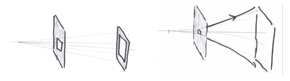
Consider a point source at some distance before an opaque screen with an aperture. According to the ray picture, the light distribution on a second screen further away from the source and parallel to the first screen is simply an enlarged copy of the aperture (see Figure \(\PageIndex{1}\)). The copy is enlarged due to the fanning out of the rays. However, this description is only accurate when the wavelength of the light is very small compared to the diameter of the aperture. If the aperture is only ten times the wavelength, the pattern is much broader due to the bending of the rays around the edge of the aperture. This phenomenon is called diffraction. It can not be explained by geometrical optics and will be studied in Chapter 6. Although it is possible to incorporate polarisation into geometrical optics, this is not standard theory and we will not consider polarisation effects in this chapter.

2.1.1.png — Figure \(\PageIndex{1}\): Light distribution on a screen due to a rectangular aperture. Left: for a large aperture, we get an enlarged copy of the aperture. Right: for an aperture that is of the order of the wavelength there is strong bending (diffraction) of the light.

Geometrical optics is accurate when the size of the objects in the system are large compared to the wavelength. It is possible to derive geometrical optics from Maxwell’s equations by expanding the electromagnetic field in a Taylor series in the wavelength and retaining only the first term of this expansion.