5.10: Fringe Visibility

Last updated
Save as PDF

Page ID: 57407

\( \newcommand{\vecs}[1]{\overset { \scriptstyle \rightharpoonup} {\mathbf{#1}} } \) \( \newcommand{\vecd}[1]{\overset{-\!-\!\rightharpoonup}{\vphantom{a}\smash {#1}}} \)\(\newcommand{\id}{\mathrm{id}}\) \( \newcommand{\Span}{\mathrm{span}}\) \( \newcommand{\kernel}{\mathrm{null}\,}\) \( \newcommand{\range}{\mathrm{range}\,}\) \( \newcommand{\RealPart}{\mathrm{Re}}\) \( \newcommand{\ImaginaryPart}{\mathrm{Im}}\) \( \newcommand{\Argument}{\mathrm{Arg}}\) \( \newcommand{\norm}[1]{\| #1 \|}\) \( \newcommand{\inner}[2]{\langle #1, #2 \rangle}\) \( \newcommand{\Span}{\mathrm{span}}\) \(\newcommand{\id}{\mathrm{id}}\) \( \newcommand{\Span}{\mathrm{span}}\) \( \newcommand{\kernel}{\mathrm{null}\,}\) \( \newcommand{\range}{\mathrm{range}\,}\) \( \newcommand{\RealPart}{\mathrm{Re}}\) \( \newcommand{\ImaginaryPart}{\mathrm{Im}}\) \( \newcommand{\Argument}{\mathrm{Arg}}\) \( \newcommand{\norm}[1]{\| #1 \|}\) \( \newcommand{\inner}[2]{\langle #1, #2 \rangle}\) \( \newcommand{\Span}{\mathrm{span}}\)\(\newcommand{\AA}{\unicode[.8,0]{x212B}}\)

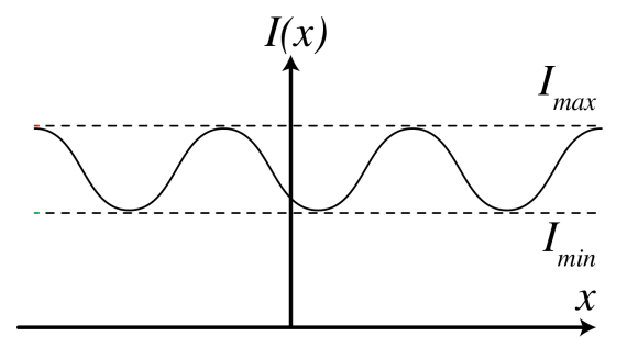
We have seen that when the interference term \(\operatorname{Re}\left\langle U_{1}^{*} U_{2}\right\rangle\) vanishes, no fringes form, while when this term is nonzero, there are fringes. The fringe visibility is expressed directly in measurable quantities (i.e. in intensities instead of fields). Given some interference intensity pattern \(I(x)\) as in Figure \(\PageIndex{1}\), the visibility is defined as \[\mathcal{V}=\frac{I_{\max }-I_{\min }}{I_{\max }+I_{\min }} . \quad \text { fringe visibility. } \nonumber \]

For example, if we have two perfectly coherent, monochromatic point sources emitting the fields \(U_{1}, U_{2}\) with intensities \(I_{1}=\left|U_{1}\right|^{2}, I_{2}=\left|U_{2}\right|^{2}\), then the interference pattern is with (5.6.13): \[I(\tau)=I_{1}+I_{2}+2 \sqrt{I_{1} I_{2}} \cos (\omega \tau+\varphi) . \nonumber \]

We then get \[I_{\max }=I_{1}+I_{2}+2 \sqrt{I_{1} I_{2}}, \quad I_{\min }=I_{1}+I_{2}-2 \sqrt{I_{1} I_{2}}, \nonumber \] \(\mathrm{SO}\) \[\mathcal{V}=\frac{2 \sqrt{I_{1} I_{2}}}{I_{1}+I_{2}} \nonumber \]

In case \(I_{1}=I_{2}\), we find \(\mathcal{V}=1\). In the opposite case, where \(U_{1}\) and \(U_{2}\) are completely incoherent, we find \[I(\tau)=I_{1}+I_{2}, \nonumber \] from which follows \[I_{\max }=I_{\min }=I_{1}+I_{2}, \nonumber \] which gives \(\mathcal{V}=0\).

5.9.1.jpg — Figure \(\PageIndex{1}\): Illustration of \(I_{\max }\) and \(I_{\min }\) of an interference pattern \(I(x)\) that determines the visibility \(\mathcal{V}\).