6.3: Angular Spectrum Method

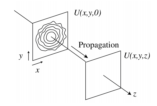
Our goal is to derive the field in some point \((x, y, z)\) with \(z=0\), given the field in the plane \(z=0\), as is illustrated in Figure \(\PageIndex{1}\). The sources of the field are assumed to be in the half space \(z<0\). One way to see how light propagates from one plane to another is by using the angular spectrum method. We decompose the field in plane waves with a two-dimensional Fourier transform. Since we know how each plane wave propagates, we can propagate each Fourier component separately and then add them all together by taking the inverse Fourier transform. Mathematically, this is described as follows: we know the field \(U(x, y, 0)\). We will write \(U_{0}(x, y)=U(x, y, 0)\) for convenience and apply a two-dimensional Fourier transform to \(U_{0}\) : \[\mathcal{F}\left(U_{0}\right)(\xi, \eta)=\iint U_{0}(x, y) e^{-2 \pi i(\xi x+\eta y)} \mathrm{d} x \mathrm{~d} y, \nonumber \] The inverse Fourier transform implies: \[\begin{aligned} U_{0}(x, y) &=\iint \mathcal{F}\left(U_{0}\right)(\xi, \eta) e^{2 \pi i(\xi x+\eta y)} \mathrm{d} \xi \mathrm{d} \eta \\ &=\mathcal{F}^{-1}\left\{\mathcal{F}\left(U_{0}\right)\right\}(x, y) . \end{aligned} \nonumber \]

Figure \(\PageIndex{1}\): Given the field \(U(x, y, 0)\), we want to find \(U\) in a point \((x, y, z)\) with \(z>0\). It is assumed that the field propagates in the positive \(z\)-direction, which means that all sources are in the region \(z<0\).

The most important properties of the Fourier transform are listed in Appendix E. By defining \(k_{x}=2 \pi \xi, k_{y}=2 \pi \(\PageIndex{2}\) \) can be written as \[U_{0}(x, y)=\frac{1}{4 \pi^{2}} \iint \mathcal{F}\left(U_{0}\right)\left(\frac{k_{x}}{2 \pi}, \frac{k_{y}}{2 \pi}\right) e^{i\left(k_{x} x+k_{y} y\right)} \mathrm{d} k_{x} \mathrm{~d} k_{y} . \nonumber \] The variables in the Fourier plane: \((\xi, \eta)\) and \(\left(k_{x}, k_{y}\right)\) are called spatial frequencies.

Equation ( \(\PageIndex{4}\) ) says that we can write \(U_{0}(x, y)=U(x, y, z=0)\) as an integral (a sum) of plane waves with wave vector \(\mathbf{k}=\left(k_{x}, k_{y}, k_{z}\right)^{T}\), each with its own weight (i.e. complex amplitude) \(\mathcal{F}\left(U_{0}\right)\left(\frac{k_{x}}{2 \pi}, \frac{k_{y}}{2 \pi}\right)\). We know how each plane wave with complex amplitude \(\mathcal{F}\left(U_{0}\right)\left(\frac{k_{x}}{2 \pi}, \frac{k_{y}}{2 \pi}\right)\) and wave vector \(\mathbf{k}=\left(k_{x}, k_{y}, k_{z}\right)^{T}\) propagates over a distance \(z>0\) \[\mathcal{F}\left(U_{0}\right)\left(\frac{k_{x}}{2 \pi}, \frac{k_{y}}{2 \pi}\right) e^{i\left(k_{x} x+k_{y} y\right)} \rightarrow \mathcal{F}\left(U_{0}\right)\left(\frac{k_{x}}{2 \pi}, \frac{k_{y}}{2 \pi}\right) e^{i\left(k_{x} x+k_{y} y+k_{z} z\right)}, \nonumber \] Therefore, the field \(U(x, y, z)\) in the plane \(z\) (for some \(z>0\) ) is given by \[U(x, y, z)=\frac{1}{4 \pi^{2}} \iint \mathcal{F}\left(U_{0}\right)\left(\frac{k_{x}}{2 \pi}, \frac{k_{y}}{2 \pi}\right) e^{i\left(k_{x} x+k_{y} y+k_{z} z\right)} \mathrm{d} k_{x} \mathrm{~d} k_{y}, \nonumber \] where \[k_{z}=\sqrt{\left(\frac{2 \pi}{\lambda}\right)^{2}-k_{x}^{2}-k_{y}^{2}}, \nonumber \] with \(\lambda\) the wavelength of the light as measured in the material (hence, \(\lambda=\lambda_{0} / n\), with \(\lambda_{0}\) the wavelength in vacuum). The sign in front of the square root in ( \PageIndex{7}\) ) could in principle be chosen negative: one would then also obtain a solution of the Helmholtz equation. The choice of the sign of \(k_{z}\) is determined by the direction in which the light propagates, which in turn depends on the location of the sources and on the convention chosen for the time dependance. We have to choose here the \(+\) sign in front of the square root because the sources are in \(z<0\) and the time dependence of time-harmonic fields is (as always in this book) given by \(e^{-i \omega t}\) with \(\omega>0\).

Eq. ( \(\PageIndex{6}\) ) can be written alternatively as \[U(x, y, z)=\mathcal{F}^{-1}\left\{\mathcal{F}\left(U_{0}\right)(\xi, \eta) e^{i k_{z} z}\right\}(x, y), \nonumber \] where now \(k_{z}\) is to be interpreted as a function of \((\xi, \eta)\) : \[k_{z}=2 \pi \sqrt{\left(\frac{1}{\lambda}\right)^{2}-\xi^{2}-\eta^{2}} . \nonumber \]

Note that one can interpret this as a diagonalisation of the propagation operator, as explained in Appendix \(\mathrm{F}\).

We can observe something interesting: if \(k_{x}^{2}+k_{y}^{2}>\left(\frac{2 \pi}{\lambda}\right)^{2}\), then \(k_{z}\) becomes imaginary, and \(\exp \left(i k_{z} z\right)\) decays exponentially for increasing \(z\) : \[\exp \left\{i\left[k_{x} x+k_{y} y+z \sqrt{\left(\frac{2 \pi n}{\lambda}\right)^{2}-k_{x}^{2}-k_{y}^{2}}\right]\right\}=e^{i\left(k_{x} x+k_{y} y\right)} e^{-z \sqrt{k_{x}^{2}+k_{y}^{2}-\left(\frac{2 \pi n}{\lambda}\right)^{2}}} . \nonumber \]

These exponentially decaying waves are evanescent in the positive \(z\)-direction. We have met evanescent waves already in the context of total internal reflection discussed in Section 1.9.5. The physical consequences of evanescent waves in the angular spectrum decomposition will be explained in Section 6.4.

The waves for which \(k_{z}\) is real have constant amplitude: only the phase changes due to propagation. These waves therefore are called propagating waves.

Remark. In homogeneous space, the scalar Helmholtz equation for every electric field component is equivalent to Maxwell’s equations and hence we may propagate each component \(E_{x}, E_{y}\) and \(E_{z}\) individually using the angular spectrum method. If the data in the plane \(z=0\) of these field components are physically consistent, the electric field thus obtained will automatically satisfy the condition that the electric field is free of divergence, i.e. \[\nabla \cdot \mathbf{E}=0 \nonumber \] everywhere in \(z>0\). This is equivalent to the statement that the electric vectors of the plane waves in the angular spectrum are perpendicular to their wave vectors. Alternatively, one can propagate only the \(E_{x^{-}}\)and \(E_{y}\)-components and afterwards determine \(E_{z}\) from the condition that ( \(\PageIndex{11}\) ) must be satisfied.