6.5: Intuition for the Spatial Fourier Transform in Optics

Since spatial Fourier transformations have played and will play a significant role in our discussion of the propagation of light, it is important to understand them not just mathematically, but also intuitively.

What happens when an object is illuminated and the reflected or transmitted light is detected at some distance from the object? Let us look at transmission for example. When the object is much larger than the wavelength, a transmission function \(\tau(x, y)\) is often defined and the field transmitted by the object is then assumed to be simply the product of the incident field and the function \(\tau(x, y)\). For example, for a hole in a metallic screen with diameter large compared to the wavelength, the transmission function would be 1 inside the hole and 0 outside. However, if the object has features of the size of the order of the wavelength, this simple model breaks down and the transmitted field must instead be determined by solving Maxwell’s equations. This is not easy, but some software packages can do it.

Now suppose that the transmitted electric field has been obtained in a plane \(z=0\) very close to the object (a distance within a fraction of a wavelength). This field is called the transmitted near field and it may have been obtained by simply multiplying the incident field with a transmission function \(\tau(x, y)\) or by solving Maxwell’s equations. This transmitted near field is a kind of footprint of the object. But it should be clear that, although it is quite common in optics to speak in terms of "imaging an object", strictly speaking we do not image an object as such, but we image the transmitted (or reflected) near field which is a kind of copy of the object. After the transmitted near field has been obtained, we apply the angular spectrum method to propagate the individual components through homogeneous matter (e.g. air) from the object to the detector plane or to an optical element like a lens.

Let \(U_{0}(x, y)=U(x, y, 0)\) be a component of the transmitted near field. The first step is to Fourier transform it, by which the field component is decomposed in plane waves. To each plane wave, characterised by the wave numbers \(k_{x}\) and \(k_{y}\), the Fourier transform assigns a complex amplitude \(\mathcal{F}\left(U_{0}\right)\left(\frac{k_{x}}{2 \pi}, \frac{k_{y}}{2 \pi}\right)\), the magnitude of which indicates how important the role is which this particular wave plays in the formation of the near field. So what can be said about the object field \(U_{0}(x, y)\), by looking at the magnitude of its spatial Fourier transform \(\left|\mathcal{F}\left(U_{0}\right)\left(\frac{k_{x}}{2 \pi}, \frac{k_{y}}{2 \pi}\right)\right|\) ?

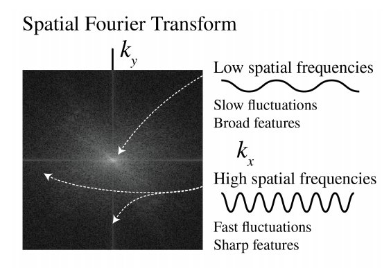
Suppose \(U_{0}(x, y)\) has sharp features, i.e. there are regions where \(U_{0}(x, y)\) varies rapidly as a function of \(x\) and \(y\). To describe these features as a combination of plane waves, these waves must also vary rapidly as a function of \(x\) and \(y\), which means that the length of their wave vectors \(\sqrt{k_{x}^{2}+k_{y}^{2}}\) must be large. Thus, the sharper the features that \(U_{0}(x, y)\) has, the larger we can expect \(\left|\mathcal{F}\left(U_{0}\right)\left(\frac{k_{x}}{2 \pi}, \frac{k_{y}}{2 \pi}\right)\right|\) to be for large \(\sqrt{k_{x}^{2}+k_{y}^{2}}\), i.e. high spatial frequencies can be expected to have large amplitude. Similarly, the slowly varying, broad features of \(U_{0}(x, y)\) are described by slowly fluctuating waves, i.e. by \(\mathcal{F}\left(U_{0}\right)\left(\frac{k_{x}}{2 \pi}, \frac{k_{y}}{2 \pi}\right)\) for small \(\sqrt{k_{x}^{2}+k_{y}^{2}}\), i.e. for low spatial frequencies. This is illustrated in Figure \(\PageIndex{1}\).

To investigate these concepts further we choose a certain field, take its Fourier transform, remove the higher spatial frequencies and then invert the Fourier transform. We then expect that the resulting field has lost its sharp features and only retains its broad features, i.e. the image is blurred. Conversely, if we remove the lower spatial frequencies but retain the higher, then the result will only show its sharp features, i.e. its contours. These effects are shown in Figure 6.5.1. Recall that when \(k_{x}^{2}+k_{y}^{2}>\left(\frac{2 \pi}{\lambda}\right)^{2}\), the plane wave decays exponentially as the field propagates. Losing these high spatial frequencies leads to a loss of resolution. Because by propagation through homogeneous space, the information contained in the high spatial frequencies corresponding to evanescent waves is lost (only exponentially small amplitudes of the evanescent waves remain), perfect imaging is impossible, no matter how well-designed an optical system is.

Propagation of light leads to irrecoverable loss of resolution.

It is this fact that motivates near-field microscopy, which tries to detect these evanescent waves by scanning close to the sample, thus obtaining subwavelength resolution, which otherwise is not possible.

So we have seen how we can guess properties of some object field \(U_{0}(x, y)\) given the amplitude of its spatial Fourier transform \(\left|\mathcal{F}\left(U_{0}\right)\left(\frac{k_{x}}{2 \pi}, \frac{k_{y}}{2 \pi}\right)\right|\). But what about the phase of \(\mathcal{F}\left(U_{0}\right)\left(\frac{k_{x}}{2 \pi}, \frac{k_{y}}{2 \pi}\right)\) ? Although one cannot really guess properties of \(U_{0}(x, y)\) by looking at the phase of \(\mathcal{F}\left(U_{0}\right)\left(\frac{k_{x}}{2 \pi}, \frac{k_{y}}{2 \pi}\right)\) the same way as we can by looking at its amplitude, it is in fact the phase that plays a larger role in defining \(U_{0}(x, y)\). This is illustrated in Figure 6.5.2: if the amplitude information of \(\mathcal{F}\left(U_{0}\right)\left(\frac{k_{x}}{2 \pi}, \frac{k_{y}}{2 \pi}\right)\) is removed, features of the original \(U_{0}(x, y)\) may still be retrieved. However, if we only know the amplitude \(\left|\mathcal{F}\left(U_{0}\right)\left(k_{x}, k_{y}\right)\right|\) but not the phase, then the original object is utterly lost. Thus, the phase of a field \(\mathcal{F}\left(U_{0}\right)\) is very important, arguably sometimes even more important than its amplitude. However, we cannot measure the phase of a field directly, only its intensity \(I=\left|\mathcal{F}\left(U_{0}\right)\right|^{2}\) from which we can calculate the amplitude \(\left|\mathcal{F}\left(U_{0}\right)\right|\). It is this fact that makes phase retrieval an entire field of study on its own: how can we find the phase of a field, given that we can only perform intensity measurements? This question is related to a new field of optics called "lensless imaging", where amplitudes and phases are retrieved from intensity measurements and the image is reconstructed computationally. Interesting as this topic may be, we will not treat it in these notes and refer instead to Master courses in optics.

Remark. The importance of the phase for the field can also be seen by looking at the plane wave expansion (6.5.3). We have seen that the field in a plane \(z=\) constant can be obtained by propagating the plane waves by multiplying their amplitudes by the phase factors \(\exp \left(i z k_{z}\right)\), which depends on the propagation distance \(z\). If one leaves the evanescent waves out of consideration (since after some distance they hardly contribute to the field anyway), it follows that only the phases of the plane waves change upon propagation, while their amplitudes (the moduli of their complex amplitudes) do not change. Yet, depending on the propagation distance \(z\), widely differing light patterns are obtained (see e.g. Figure 6.5.4).

Another aspect of the Fourier transform is the uncertainty principle. It states that many waves of different frequencies have to be added to get a function that is confined to a small space. Stated differently, if \(U(x, y)\) is confined to a very small region, then \(\mathcal{F}(U)\left(k_{x}, k_{y}\right)\) must be very spread out. This can also be illustrated by the scaling property of the Fourier transform: \[\text { if } h(x)=f(a x) \text { then } \mathcal{F}(h)\left(\frac{k_{x}}{2 \pi}\right)=\frac{1}{|a|} \mathcal{F}(f)\left(\frac{k_{x}}{2 \pi a}\right) \text {, } \nonumber \] which simply states that the more \(h(x)\) is squeezed by increasing \(a\), the more its Fourier transform \(\mathcal{F}(h)\) spreads out. This principle is illustrated in Figure 6.5.3. The uncertainty principle is familiar from quantum physics where it is stated that a particle cannot have both a definite momentum and a definite position. In fact, this is just one particular manifestation of the uncertainty principle just described. A quantum state \(|\psi\rangle\) can be described in the position basis \(\psi_{x}(x)\) as well as in the momentum basis \(\psi_{p}(p)\). The basis transformation that links these two expressions is the Fourier transform \[\psi_{p}(p)=\mathcal{F}\left\{\psi_{x}(x)\right\}(p) . \nonumber \]

Figure \(\PageIndex{1}\): A qualitative interpretation of spatial Fourier transforms. The low spatial frequencies (i.e. small \(\sqrt{k_{x}^{2}+k_{y}^{2}}\) ) represent slow fluctuations, and therefore contribute to the broad features of the real-space object. The high spatial frequencies (i.e. large \(\sqrt{k_{x}^{2}+k_{y}^{2}}\) ) fluctuate rapidly, and can therefore form sharp features in the real-space object.

Hence, the two are obviously subject to the uncertainty principle! In fact, any two quantum observables which are related by a Fourier transform (also called conjugate variables), such as position and momentum, obey this uncertainty relation.

The uncertainty relation roughly says:

If a function \(f(x)\) has width \(\Delta x\), its Fourier transform has a width \(\Delta k_{x} \approx 2 \pi / \Delta x\).

Since after propagation over a distance \(z\), the evanescent waves do not contribute to the Fourier transform of the field, it follows that this Fourier transform has maximum width \(\Delta k_{x}=k\). By the uncertainty principle it follows that after propagation, the minimum width of the field is \(\Delta x, \Delta y \approx 2 \pi / k=\lambda\).

The minimum feature size of a field after propagation is of the order of the wavelength.

This poses a fundamental limit to resolution given by the wavelength of the light.