6.6: Fresnel and Fraunhofer Approximations

The Fresnel and Fraunhofer approximation are two approximations of the Rayleigh-Sommerfeld integral (6.13). The approximations are based on the assumption that the field has propagated over a sufficiently large distance \(z\). In the Fraunhofer approximation, \(z\) has to be very large, i.e. much larger than for the Fresnel approximation to hold. Putting it differently: in order of most accurate to least accurate (i.e. only valid for large propagation distances), the diffraction integrals would rank as:

[Most accurate] \(\quad\) Rayleigh-Sommerfeld \(\rightarrow\) Fresnel \(\rightarrow\) Fraunhofer \(\quad\) [Least accurate].

Figure \(\PageIndex{1}\): Demonstration of the roles of different spatial frequencies. By removing the high spatial frequencies, only the broad features of the image remain: we lose resolution. If the low spatial frequencies are removed, only the sharp features (i.e. the contours) in the image remain.

Figure \(\PageIndex{2}\): Demonstration of the role of the phase of the spatial Fourier transform. If the amplitude information is removed, but phase information is kept, some features of the original image are still recognizable. However, if the phase information is removed but amplitude information is kept, the original image is completely lost.

6.5.1 Fresnel Approximation

For both approximations, we assume that \(z\) in Eq. (6.3.1) is so large that in the denominator we can approximate \(r \approx z\) \[\begin{aligned} U(x, y, z) &=\frac{1}{i \lambda} \iint U_{0}\left(x^{\prime}, y^{\prime}\right) \frac{z}{r} \frac{e^{i k r}}{r} \mathrm{~d} x^{\prime} \mathrm{d} y^{\prime} \\ & \approx \frac{1}{i \lambda z} \iint U_{0}\left(x^{\prime}, y^{\prime}\right) e^{i k r} \mathrm{~d} x^{\prime} \mathrm{d} y^{\prime} . \end{aligned} \nonumber \]

The reason why we can not apply the same approximation for \(r\) in the exponent, is that there \(r\) is multiplied by \(k=2 \pi / \lambda\), which is very large, so any error introduced by approximating \(r\) would be magnified significantly by \(k\) and then can lead to a completely different value of \(\exp (i k r)=\cos (k r)+i \sin (k r)\). To approximate \(r\) in the exponent \(\exp (i k r)\) we must be more careful and instead apply a Taylor expansion. Recall that \[\begin{aligned} r &=\sqrt{\left(x-x^{\prime}\right)^{2}+\left(y-y^{\prime}\right)^{2}+z^{2}} \\ &=z \sqrt{\frac{\left(x-x^{\prime}\right)^{2}+\left(y-y^{\prime}\right)^{2}}{z^{2}}+1} . \end{aligned} \nonumber \]

We know that for a small number \(s\) we can expand \[\sqrt{s+1}=1+\frac{s}{2}-\frac{s^{2}}{8}+\ldots . \nonumber \]

Since we assumed that \(z\) is large, \(\frac{\left(x-x^{\prime}\right)^{2}+\left(y-y^{\prime}\right)^{2}}{z^{2}}\) is small, so we can expand \[\begin{aligned} r &=z \sqrt{\frac{\left(x-x^{\prime}\right)^{2}+\left(y-y^{\prime}\right)^{2}}{z^{2}}+1} \\ & \approx z\left(1+\frac{\left(x-x^{\prime}\right)^{2}+\left(y-y^{\prime}\right)^{2}}{2 z^{2}}\right) \\ &=z+\frac{\left(x-x^{\prime}\right)^{2}+\left(y-y^{\prime}\right)^{2}}{2 z}, \quad \text { Fresnel approximation. } \end{aligned} \nonumber \]

With this approximation, we arrive at the Fresnel diffraction integral, which can be written in the following equivalent forms: \[\begin{aligned} U(x, y, z) & \approx \frac{e^{i k z}}{i \lambda z} \iint U_{0}\left(x^{\prime}, y^{\prime}\right) e^{\frac{i k}{2 z}\left[\left(x-x^{\prime}\right)^{2}+\left(y-y^{\prime}\right)^{2}\right]} \mathrm{d} x^{\prime} \mathrm{d} y^{\prime} \\ &=\frac{e^{i k z} e^{\frac{i k\left(x^{2}+y^{2}\right)}{2 z}}}{i \lambda z} \iint U_{0}\left(x^{\prime}, y^{\prime}\right) e^{\frac{i k\left(x^{\prime 2}+y^{\prime 2}\right)}{2 z}} e^{-i k\left(\frac{x}{z} x^{\prime}+\frac{y}{z} y^{\prime}\right)} \mathrm{d} x^{\prime} \mathrm{d} y^{\prime} \\ &=\frac{e^{i k z} e^{\frac{i k\left(x^{2}+y^{2}\right)}{2 z}}}{i \lambda z} \mathcal{F}\left\{U_{0}\left(x^{\prime}, y^{\prime}\right) e^{\frac{i k\left(x^{\prime 2}+y^{\prime 2}\right)}{2 z}}\right\}\left(\frac{x}{\lambda z}, \frac{y}{\lambda z}\right) . \end{aligned} \nonumber \]

Especially the last expression is interesting, because it shows that

The Fresnel integral is the Fourier transform of the field \(U_{0}\left(x^{\prime}, y^{\prime}\right)\) multiplied by the Fresnel propagator \(\exp \left(\frac{i k\left(x^{\prime 2}+y^{\prime 2}\right)}{2 z}\right)\).

Note that this propagator depends on the distance of propagation \(z\).

Remark. By Fourier transforming \((\(\PageIndex{6}\))\), one gets the plane wave amplitudes of the Fresnel integral. It turns out that these amplitudes are equal to \(\mathcal{F}\left(U_{0}\right)\) multiplied by a phase factor. This phase factor is a paraxial approximation of the exact phase factor given by \(\exp \left(i z k_{z}\right)\), i.e. it contains as exponent the parabolic approximation of \(k_{z}\). Therefore the Fresnel approximation is also called the paraxial approximation. In fact, it can be shown that the Fresnel diffraction integral is a solution of the paraxial wave equation and conversely, that every solution of the paraxial wave equation can be written as a Fresnel diffraction integral.

6.5.2 Fraunhofer Approximation

For the Fraunhofer approximation, we will make one further approximation to \(r\) in \(\exp (i k r)\) \[\begin{aligned} r & \approx z+\frac{\left(x-x^{\prime}\right)^{2}+\left(y-y^{\prime}\right)^{2}}{2 z} \text { Fresnel approximation } \\ & \approx z+\frac{x^{2}+y^{2}-2 x x^{\prime}-2 y y^{\prime}}{2 z} \text { Fraunhofer approximation. } \end{aligned} \nonumber \]

Hence we have omitted the quadratic terms \(x^{\prime 2}+y^{\prime 2}\), and compared with respect the Fresnel diffraction integral, we simply omit the factor \(\exp \left(\frac{i k\left(x^{\prime 2}+y^{\prime 2}\right)}{2 z}\right)\) to obtain the Fraunhofer diffraction integral: \[U(x, y, z) \approx \frac{e^{i k z} e^{\frac{i k\left(x^{2}+y^{2}\right)}{2 z}}}{i \lambda z} \mathcal{F}\left(U_{0}\right)\left(\frac{x}{\lambda z}, \frac{y}{\lambda z}\right) \nonumber \]

This leads to the following important observation:

The Fraunhofer far field of \(U_{0}\left(x^{\prime}, y^{\prime}\right)\) is simply its Fourier transform with an additional quadratic phase factor.

Note that the coordinates for which we have to evaluate \(\mathcal{F}\left(U_{0}\right)\) scale with \(1 / z\), and the overall field \(U(x, y, z)\) is proportional to \(1 / z\). This means that as you choose \(z\) larger (i.e. you propagate the field further), the field simply spreads out without changing its shape, and its amplitude goes down. Stated differently, apart from the factor \(1 / z\) in front of the integral, the Fraunhofer field only depends on the angles \(x / z\) amd \(y / z\). Therefore the field diverges as the propagation distance \(z\) increases.

Eventually, for sufficiently large propagation distances, i.e. in the Fraunhofer limit, light always spreads out without changing the shape of the light distribution.

Remarks.

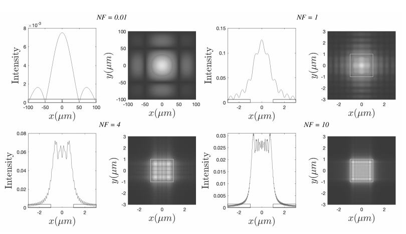
1. The Fresnel integral is, like the Fraunhofer integral, also a Fourier transform, evaluated in spatial frequencies which depend on the point of observation: \[\xi=\frac{x}{\lambda z}, \quad \eta=\frac{y}{\lambda z} . \nonumber \] However, in contrast to the Fraunhofer integral, the Fresnel integral depends additionally in a different way on the propagation distance \(z\), namely through the epxonent of the propagator in the integrand. This is the reason that the Fresnel integral does not merely depend on \(z\) through the ratios \(x / z\) and \(y / z\) but in a more complicated manner. Therefore the Fresnel integral gives quite diverse patterns depending on the value of the propagation distance \(z\), as is shown in Figure \(\PageIndex{4}\).
2. Let \(f_{a, b}(x, y)=f(x-a, y-b)\) be the function obtained from \(f\) by translation. From the general property of the Fourier transform: \[\mathcal{F}\left(f_{a, b}\right)(\xi, \eta)=e^{-2 \pi i(\xi a+\eta b)} \mathcal{F}(f)(\xi, \eta) . \nonumber \] Hence, when the field \(U_{0}\) is translated, the intensity in the Fraunhofer far field is not changed. In contrast, due to the additional quadratic phase factor in the integrand of the Fresnel integral, the intensity of the Fresnel field in general changes when \(U_{0}\) is translated.
3. Suppose that \(U_{0}\) is the field immediately behind an aperture \(\mathcal{A}\) with diameter \(D\) in an opaque screen. It can then be shown that points \((x, y, z)\) of observation, for which the Fresnel and Fraunhofer diffraction integrals are sufficiently accurate, satisfy: \[\begin{aligned} &\frac{z}{\lambda}>\left(\frac{\max _{\left(x^{\prime}, y^{\prime}\right) \in \mathcal{A}} \sqrt{\left(x-x^{\prime}\right)^{2}+\left(y-y^{\prime}\right)^{2}}}{\lambda}\right)^{4 / 3} \text {, Fresnel } \\ &\frac{z}{\lambda}>\left(\frac{D}{\lambda}\right)^{2} \text {, Fraunhofer } \end{aligned} \nonumber \] Suppose that \(D=1 \mathrm{~mm}\) and the wavelength is green light: \(\lambda=550 \mathrm{~nm}\), then Fraunhofer’s approximation is accurate if \(z>2 \mathrm{~m}\). The inequality ( \(\PageIndex{6}\) ) is sufficient for the Fresnel formula to be accurate, but it is not always necessary. Often the Fresnel approximation is already accurate for smaller propagation distances.
4. The points of observation where the Fraunhofer formulae can be used must in any case satisfy: \[\frac{x}{z}<1, \quad \frac{y}{z}<1 . \nonumber \] When \(x / z>1\), the spatial frequency \(k_{x}=\frac{2 \pi x}{z \lambda}>k\) associated with this point corresponds to an evanescent wave. An evanescent wave obviously cannot contribute to the Fraunhofer far field because it exponentially decreases with distance \(z\).
5. In any expression for an optical field, one may always omit factors of constant phase, i.e. an overall phase which does not depend on position. If one is only interested in the field in certain planes \(z=\) constant, then a factor like \(\exp (i k z)\) may also be omitted. Further, in some cases also a position dependent phase factor in front of the Fresnel and Fraunhofer diffraction integrals is omitted, namely when only the intensity is of interest. In exercises it is usually mentioned that this factor may be omitted: if this is not stated, it should be retained in the formulae.

Figure \(\PageIndex{3}\): Demonstration of the uncertainty principle. The more confined \(U(x, y)\) is, the larger the spread of \(\mathcal{F}(U)\left(\frac{k_{x}}{2 \pi}, \frac{k_{y}}{2 \pi}\right)\).

Figure \(\PageIndex{4}\): Example of intensities of Fresnel fields of a square aperture, shown as contours and in cross section for different distances which increase from the lower right to the upper left. The upper left pattern is equal to the Fraunhofer pattern. \(N_{F}=D^{2} / \lambda z\) is the Fresnel number and \(\lambda=600 \mathrm{~nm} .\)

6.5.3 Examples of Fresnel and Fraunhofer fields

Fresnel approximation of the field of two point sources.

Consider two point sources in \(\mathbf{r}_{s}^{+}=(a / 2,0,0)\) and \(\mathbf{r}_{s}^{-}=(-a / 2,0,0)\). The fields of each of them in a point \(\mathbf{r}=(x, y, z)\) are given by (5.6.2) \[U_{\pm}(\mathbf{r})=\frac{e^{i k\left|\mathbf{r}-\mathbf{r}_{s}^{\pm}\right|}}{\left|\mathbf{r}-\mathbf{r}_{s}^{\pm}\right|} \nonumber \]

We apply the Fresnel approximation for large \(z\) : \[\begin{aligned} \left|\mathbf{r}-\mathbf{r}_{s}^{\pm}\right| &=z \sqrt{1+\frac{(x \mp a / 2)^{2}+y^{2}}{z^{2}}} \\ & \approx z+\frac{(x \mp a / 2)^{2}+y^{2}}{2 z} \\ &=z+\frac{x^{2}+y^{2}+a^{2} / 4}{2 z} \mp \frac{a x}{2 z} . \end{aligned} \nonumber \]

Hence, \[U_{\pm}(\mathbf{r}) \approx \frac{e^{i k z}}{z} e^{i k \frac{x^{2}+y^{2}}{2 z}} e^{i k \frac{a^{2}}{8 z}} e^{\mp i k \frac{a x}{2 z}}, \nonumber \] where in the denominator we replaced \(\left|\mathbf{r}-\mathbf{r}_{s}^{\pm}\right|\)by \(z\). Note that the Fraunhofer approximation amounts to \(e^{i k a^{2} /(8 z)} \approx 1\) while the phase factor \(e^{i k \frac{x^{2}+y^{2}}{2 z}}\) remains. The intensity on a screen \(z=\) constant of the total field is \[\begin{aligned} I_{\text {tot }}(\mathbf{r}) &=\left|U_{+}(\mathbf{r})+U_{-}(\mathbf{r})\right|^{2}=\frac{1}{z^{2}}\left|e^{-i k \frac{a x}{2 z}}+e^{i k \frac{a x}{2 z}}\right|^{2} \\ &=\frac{2}{z^{2}}\left[1+\cos \left(2 \pi \frac{a x}{\lambda z}\right)\right] \end{aligned} \nonumber \]

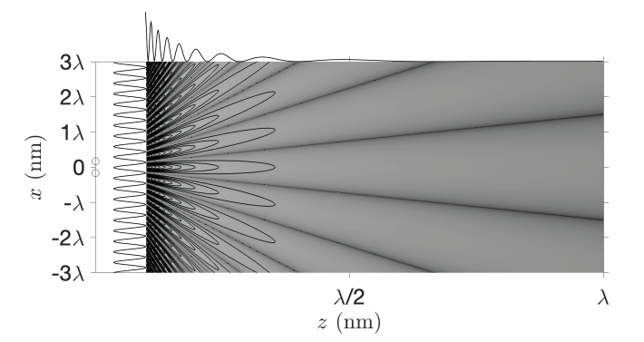
It is seen that the intensity results from the interference of two plane waves: \(\exp [\pm i k a x /(\lambda z)]\) and is given by a cosine function (see Figure \(\PageIndex{5}\) ). Note that for two point sources, the intensity pattern is the same in the Fresnel and the Fraunhofer approximation. However, this is special for two point sources: when more than two point sources are considered, the Fresnel and Fraunhofer patterns are different. The intensity pattern is independent of \(y\), and vanishes on lines \[\frac{x}{z}=(2 m+1) \frac{\lambda}{2 a} \nonumber \] and has maxima on lines \[\frac{x}{z}=m \frac{\lambda}{a}, \nonumber \] for integer \(m\).

Fraunhofer field of a rectangular aperture in a screen.

Let the screen be \(z=0\) and the aperture be given by \(-a / 2<x<a / 2,-b / 2<y<b / 2\). The transmission function \(\tau(x, y)\) is: \[\tau(x, y)=1_{[-a / 2, a / 2]}(x) 1_{[-b / 2, b / 2]}(y), \nonumber \] where \[1_{[-a / 2, a / 2]}(x)=\left\{\begin{array}{l} 1, \text { if }-\frac{a}{2} \leq x \leq \frac{a}{2}, \\ 0, \text { otherwise }, \end{array}\right. \nonumber \] and similarly for \(1_{[-b / 2, b / 2]}(y)\). Let the slit be illuminated by a perpendicular incident plane wave with unit amplitude. Then the field immediately behind the screen is: \[U_{0}(x, y)=\tau(x, y)=1_{[-a / 2, a / 2]}(x) 1_{[-b / 2, b / 2]}(y), \nonumber \] We have \[\begin{aligned} \mathcal{F}\left(1_{[-a / 2, a / 2]}\right)(\xi) &=\int_{-a / 2}^{a / 2} e^{-2 \pi i \xi x} \mathrm{~d} x \\ &=\frac{e^{\pi i a \xi}-e^{-\pi i a \xi}}{2 \pi i \xi} \\ &=a \frac{\sin (\pi a \xi)}{\pi a \xi} \\ &=a \operatorname{sinc}(\pi a \xi), \end{aligned} \nonumber \] where \(\operatorname{sinc}(u)=\sin (u) / u\). Hence, \[\mathcal{F}\left(U_{0}\right)\left(\frac{x}{\lambda z}, \frac{y}{\lambda z}\right)=a b \operatorname{sinc}\left(\frac{\pi a x}{\lambda z}\right) \operatorname{sinc}\left(\frac{\pi b y}{\lambda z}\right) . \nonumber \] The Fraunhofer far field of a rectangular aperture in a plane at large distance \(z\) is obtained by substituting ( \(\PageIndex{25}\) ) into ( \(\PageIndex{9}\) ).

Figure \(\PageIndex{5}\): Fraunhofer intensity pattern of two coherent point sources \(200 \mathrm{~nm}\) apart (circles), of equal strength for \(\lambda=600 \mathrm{~nm}\).

Remarks.

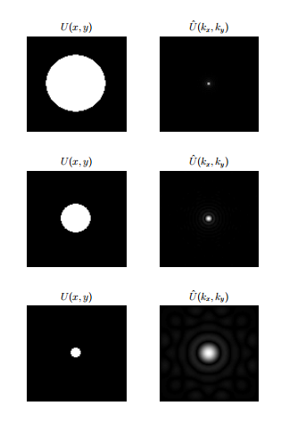
1. The first zero along the \(x\)-direction from the centre \(x=0\) occurs for \[x=\pm \frac{\lambda z}{a} . \nonumber \] The distance between the first two zeros along the \(x\)-axis is \(2 \lambda z / a\) and is thus larger when the width along the \(x\)-direction of the aperture is smaller.
2. The inequalities ( \(\PageIndex{14}\) ) imply that when \(a<\lambda\), the far field pattern does not have any zeros as function of \(x\). It is then difficult or even impossible to deduce the width \(a\) from the Fraunhofer intensity. This is an illustration of the fact that information about sizes less than the wavelength cannot propagate to the far field.
3. As shown in Figure \(\PageIndex{6}\), the Fraunhofer diffraction pattern as function of diffraction angle is narrowest in the direction in which the aperture is widest.

Figure \(\PageIndex{6}\): Fraunhofer diffraction pattern of a rectangular aperture in an opaque screen. In a) the width of the aperture in the \(y\)-direction is twice that in the \(x\) direction. In b) the width in the \(y\)-direction is 10 times that in the \(x\)-direction.

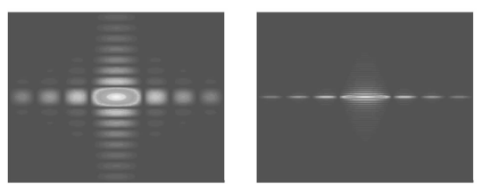
Periodic array of slits

We can now predict what the diffraction pattern of a series of slits of finite width will look like. It follows from the Fraunhofer pattern of a single rectangular aperture that, if the sides parallel to a a direction are very long, the Fraunhofer diffraction pattern as function of angle in that direction is very narrow. In Figure \(\PageIndex{6}\) b the Fraunhofer diffraction pattern of a rectangular aperture is shown, of which the width in the \(y\)-direction is 10 times that in the \(x\)-direction. The diffraction pattern is then strongly concentrated along the \(x\)-axis. If we only consider the Fraunhofer pattern for \(y / z=0\) while still considering it as a function of \(x / z\), it suffices to compute the Fourier transform only with respect to \(x\). The problem then becomes a diffraction problem for a one-dimensional slit.

We consider now an array of such slits of which the long sides are all parallel to the \(y\)-axis and neglect from now on the \(y\)-variable. Suppose \(W_{\text {slit }}(x)\) is a block function describing the transmission function of a single slit. We define the Dirac comb by \[\mathrm{II}_{\Delta}(x)=\sum_{m=-\infty}^{\infty} \delta(x-m \Delta) . \nonumber \]

Then the transmission function of an infinite series of slits with finite width is given by the convolution \(\mathrm{II}_{\Delta}(x) * W_{\text {slit }}(x)\). To make the number of slits finite, we multiply the expression with another block function \(W_{\text {array }}(x)\) and get \[\tau(x)=\left(\mathrm{II}_{\Delta}(x) * W_{\text {slit }}(x)\right) W_{\text {array }}(x) . \nonumber \]

The diffraction pattern in the far field is given by the Fourier transform of the transmitted near field. If the incident illumination is a perpendicular plane wave with unit amplitude, the transmitted near field is simply \(\tau(x)\). Using the fact that convolutions in real space correspond to products in Fourier space and vice versa, and using the fact that \[\mathcal{F}\left\{\mathrm{W}_{\Delta}(x)\right\}=(1 / \Delta) \mathrm{W}_{1 / \Delta}(\xi), \nonumber \] see Appendix (E.9) and (E.10), we find \[\mathcal{F}(\tau)=\frac{1}{\Delta}\left[\mathrm{W}_{1 / \Delta} \mathcal{F}\left(W_{\text {slit }}\right)\right] * \mathcal{F}\left(W_{\text {array }}\right). \nonumber \]

If the slit has width \(a\) : \[\begin{aligned} \frac{1}{\Delta} \mathrm{I}_{1 / \Delta} \mathcal{F}\left(W_{\text {slit }}\right)(\xi) &=\frac{a}{\Delta} \sum_{m=-\infty}^{\infty} \delta\left(\xi-\frac{m}{\Delta}\right) \operatorname{sinc}(\pi a \xi) \\ &=\frac{a}{\Delta} \sum_{m=-\infty}^{\infty} \operatorname{sinc}\left(m \pi \frac{a}{\Delta}\right) \delta\left(\xi-\frac{m}{\Delta}\right) . \end{aligned} \nonumber \]

If the total width of the array is \(A\), then \[\mathcal{F}\left(W_{\text {array }}\right)(\xi)=A \operatorname{sinc}(\pi A \xi), \nonumber \] and we conclude that \[\mathcal{F}(\tau)(\xi)=\frac{a A}{\Delta} \sum_{m=-\infty}^{\infty} \operatorname{sinc}\left(m \pi \frac{a}{\Delta}\right) \operatorname{sinc}\left(\pi A\left(\xi-\frac{m}{\Delta}\right)\right) . \nonumber \]

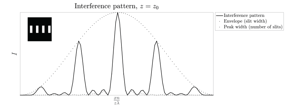
The Fraunhofer field of the array of slits is (omitting the quadratic phase factor): \[\mathcal{F}(\tau)\left(\frac{x}{\lambda z}\right)=\frac{a A}{\Delta} \sum_{m=-\infty}^{\infty} \operatorname{sinc}\left(m \pi \frac{a}{\Delta}\right) \operatorname{sinc}\left(\pi A\left(\frac{x}{\lambda z}-\frac{m}{\Delta}\right)\right) . \nonumber \]

For the directions \[\frac{x}{z}=\theta_{m}=\frac{m \lambda}{\Delta}, \quad m=0, \pm 1, \pm 2, \ldots, \quad \text { diffraction orders } \nonumber \] the field has local maxima (peaks). These directions are called diffraction orders. Note that as explained above, there should hold: \(x / z<1\) in the Fraunhofer far field, which sets a limit to the number of the diffracted orders that occur. This limit depends on the period and the wavelength and is defined by: \[|m| \leq \Delta / \lambda . \nonumber \]

Hence, the larger the ratio of the period and the wavelength, the more diffraction orders.

The width of a diffraction order is given by the width of the function ( \(\PageIndex{31}\) ), i.e. it is given by \[\Delta \theta=\frac{\lambda}{A}, \quad \text { angular width of a diffraction order. } \nonumber \]

Hence, the larger \(A\), i.e. the more slits there are in the array, the narrower the peaks into which the energy is diffracted.

The property ( \(\PageIndex{34}\) ) that the angles of diffraction of the orders depend on wavelength is used to separate wavelengths. Grating spectrometers use periodic structures such as this array of slits to very accurately separate and measure wavelengths. For example, for a grating with 1000 periods one can obtain a resolution of \(\Delta \lambda / \lambda=10^{-3}\).

The amplitudes of the diffracted orders: \[\operatorname{sinc}\left(m \pi \frac{a}{\Delta}\right), \nonumber \] are determined by the width of the slits. Hence the envelope (i.e. large features) of the Fraunhofer diffraction pattern is determined by the small-scale properties of the array, namely the width of the slits. This is illustrated in Figure \(\PageIndex{7}\). Remark. A periodic row of slits is an example of a diffraction grating. A grating is a periodic structure, i.e. the permittivity is a periodic function of position. Structures can be periodic in one, two and three directions. A crystal acts as a three-dimensional grating whose period is the period of the crystal, i.e. a few Angstrom. Electromagnetic waves of wavelength equal to one Angstrom or less are called x-rays. When a beam of x-rays illuminates a crystal, a detector in the far field measures the Fraunhofer diffraction pattern given by the intensity of the Fourier transform of the refracted near field. These diffraction orders of crystals for x-rays where discovered by Von Laue and are used to study the atomic structure of crystals.

Figure \(\PageIndex{7}\): An illustration of a diffraction pattern of a series of four slits.