6.8: Fourier Optics

In this section we apply diffraction theory to a lens. We consider in particular the focusing of a parallel beam and the imaging of an object.

6.8.1 Focusing of a Parallel Beam

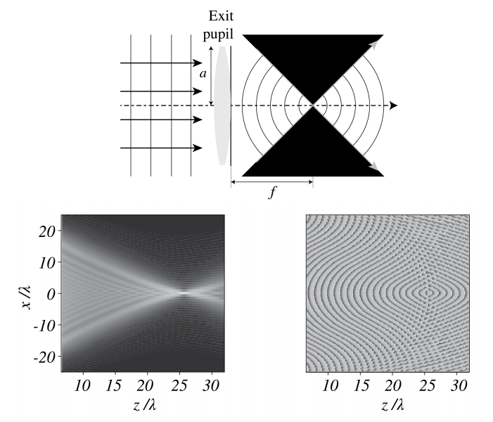
A lens induces a local phase change to an incident field which is proportional to its local thickness. Let a plane wave which propagates parallel to the optical axis be incident on the lens. According to Gaussian geometrical optics, the incident rays are parallel to the optical axis and are all focused into the focal point. According to the Principle of Fermat, all rays have travelled the same optical distance when they intersect in the focal point where constructive interference occurs and the intensity is maximum. In the focal region, the wavefronts are spheres with centre the focal point which are cut off by the cone with the focal point as top and opening angle \(2 a / f\), as shown in Figure \(\PageIndex{1}\). Behind the focal point, there is a second cone where there are again spherical wavefronts, but there the light is of course propagating away from the focal point. According to Gaussian geometrical optics it is in image space completely dark outside of the two cones in Figure \(\PageIndex{1}\). However, as we will show, in diffraction optics this is not true.

We assume that the lens is thin and choose as origin of the coordinate system the centre of the thin lens with the positive \(z\)-axis along the optical axis. Let \(f\) be the focal distance according to Gaussian geometrical optics. Then \((0,0, f)\) is the focal point. Let \((x, y, z)\) be a point between the lens and the focal point. According to geometrical optics the field in \((x, y, z)\) is \[\begin{array}{cc} \frac{e^{-i k \sqrt{x^{2}+y^{2}+(z-f)^{2}}-i \omega t}}{\sqrt{x^{2}+y^{2}+(z-f)^{2}}}, & \text { if }(x, y, z) \text { is inside the cone, } \\ 0, & \text { if }(x, y, z) \text { is outside the cone, } \end{array} \nonumber \] where we have included the time-dependence. Indeed the surfaces of constant phase: \[-\sqrt{x^{2}+y^{2}+(z-f)^{2}}-\omega t=\text { constant, } \nonumber \] are spheres with centre the focal point which for increasing time converge to the focal point, while the amplitude of the field increases in proportion to the reciprocal of the distance to the focal point so that energy is preserved.

Remark. For a point \((x, y, z)\) to the right of the focal point, the spherical wave fronts propagate away from the focal point and therefore for \(z>f,-i k\) should be replaced by \(+i k\) in the exponent in \(\PageIndex{1}\).

The exit pupil of the lens is in the plane \(z=0\) where according to ( \(\PageIndex{1}\) ) the field is \[1_{\odot_{a}}(x, y) \frac{e^{-i k \sqrt{x^{2}+y^{2}+f^{2}}}}{\sqrt{x^{2}+y^{2}+f^{2}}}, \nonumber \] where the time dependence has been omitted and \(1_{\odot_{a}}(x, y)=\) \begin{cases}1 & \text { if } x^{2}+y^{2}<a^{2}, \\ 0 & \text { otherwise }\end{cases} i.e. \(1_{\odot_{a}}(x, y)=1\) for \((x, y)\) in the exit pupil of the lens and \(=0\) otherwise.

In diffraction optics we compute the field in the focal region using diffraction integrals instead of using ray tracing. Hence, the modification introduced by diffraction optics is due to the more accurate propagation of the field from the exit pupil to the focal region.

If \(a / f\) is sufficiently small, we may replace the distance \(\sqrt{x^{2}+y^{2}+f^{2}}\) between a point in the exit pupil and the focal point in the denominator of ( \(\PageIndex{2}\) ) by \(f\). This is not allowed in the exponent, however, because of the multiplication by the large wave number \(k\). In the exponent we therefore use instead the first two terms of the Taylor series, 6.5.4: \[\sqrt{x^{2}+y^{2}+f^{2}}=f \sqrt{1+\frac{x^{2}+y^{2}}{f^{2}}} \approx f+\frac{x^{2}+y^{2}}{2 f}, \nonumber \] which is valid for \(a / f\) sufficiently small. Then ( \(\PageIndex{2}\) ) becomes: \[1 \odot_{a}(x, y) e^{-i k \frac{x^{2}+y^{2}}{2 f}}, \nonumber \] where we dropped the constant factors \(e^{i k f}\) and \(1 / f\). For a general incident field \(U_{0}(x, y)\) in the entrance pupil, the lens applies a transformation such that the field in the exit plane becomes: \[U_{0}(x, y) \rightarrow U_{0}(x, y) 1_{\odot_{a}}(x, y) e^{-i k \frac{x^{2}+y^{2}}{2 f}}, \nonumber \] transformation applied by a lens between its entrance and exit plane.

The function that multiplies \(U_{0}(x, y)\) is the transmission function of the lens: \[\tau_{lens }(x, y)=1\odot_{a}(x, y) e^{-i k \frac{x^{2}+y^{2}}{2 f}} . \nonumber \]

This result makes sense: in the centre \((x, y)=0\) the lens is thickest, so the phase is shifted the most (but we can define this phase shift to be zero because only phase differences matter, not absolute phase). As is indicated by the minus-sign in the exponent, the further you move away from the centre of the lens, the less the phase is shifted. For shorter \(f\), the lens focuses more strongly, so the phase shift changes more rapidly as a function of the radial coordinate. Note that transmission function ( \(\PageIndex{7}\) ) has modulus 1 so that energy is conserved. We use the Fresnel diffraction integral (6.5.6) to propagate the field ( \(\PageIndex{6}\) ) to the focal region: \[U(x, y, z)=\frac{e^{i k z} e^{\frac{i k\left(x^{2}+y^{2}\right)}{2 z}}}{i \lambda z} \mathcal{F}\left\{U_{0}\left(x^{\prime}, y^{\prime}\right) 1\odot_{a}\left(x^{\prime}, y^{\prime}\right) e^{i k \frac{x^{\prime 2}+y^{\prime 2}}{2}}\left(\frac{1}{z}-\frac{1}{f}\right)\right\}\left(\frac{x}{\lambda z}, \frac{y}{\lambda z}\right) . \nonumber \]

The intensity \(I=|U|^{2}\) is shown at the bottom left of Figure \(\PageIndex{1}\). It is seen that the intensity does not monotonically increase for decreasing distance to the focal point. Instead, secondary maxima are seen along the optical axis. Also the boundary of the light cone is not sharp, as predicted by geometrical optics, but diffuse. The bottom right of Figure \(\PageIndex{1}\) shows the phase in the focal region. The wave fronts are close to but not exactly spherical inside the cones.

Figure \(\PageIndex{1}\): Top: wavefronts of the incident plane wave and the focused field according to Gaussian geometrical optics. There is no light outside of the two cones. Bottom left: amplitude as predicted by diffraction optics. The boundary of the cones is diffuse and it is not absolutely dark outside of the cones. Furthermore, the intensity does not increase monotonically with decreasing distance to the focal point, as predicted by geometrical optics. Bottom right: phase of the focused field as predicted by diffraction optics.

For points in the back focal plane of the lens, i.e. \(z=f\), we have \[U(x, y, f)=\frac{e^{i k f} e^{\frac{i k\left(x^{2}+y^{2}\right)}{2 f}}}{i \lambda f} \mathcal{F}\left\{U_{0}\left(x^{\prime}, y^{\prime}\right) 1\odot_{a}\left(x^{\prime}, y^{\prime}\right)\right\}\left(\frac{x}{\lambda f}, \frac{y}{\lambda f}\right), \nonumber \] which is the same as the Fraunhofer integral! Thus, the field in the focal plane according to Gaussian geometrical optics is in diffraction optics identical to the far field of the field in the entrance pupil of the lens, or to put it differently:

The field in the entrance pupil of the lens and the field in the focal plane are related by a Fourier transform (apart from a quadratic phase factor in front of the integral).

It can be shown that the fields in the front focal plane \(U(x, y,-f)\) and the back focal plane \(U(x, y, f)\) are related exactly by a Fourier transform, i.e. without the additional quadratic phase factor.

So a lens performs a Fourier transform. Let us see if that agrees with some of the facts we know from geometrical optics.

1. We know from Gaussian geometrical optics that if we illuminate a lens with rays parallel to the optical axis, these rays all intersect in the focal point. This corresponds with the fact that for \(U_{0}(x, y)=1\) (i.e. plane wave illumination, neglecting the finite aperture of the lens, i.e. neglecting diffraction effects due to the finite size of the pupil), its Fourier transform is a delta peak:

\[\mathcal{F}\left(U_{0}\right)\left(\frac{k_{x}}{2 \pi}, \frac{k_{y}}{2 \pi}\right)=\delta\left(\frac{k_{x}}{2 \pi}\right) \delta\left(\frac{k_{y}}{2 \pi}\right), \nonumber \] which represents the perfect focused spot (without diffraction).

2. If in Gaussian geometrical optics we illuminate a lens with tilted parallel rays of light (a plane wave propagating in an oblique direction), then the point in the back focal plane where the rays intersect is laterally displaced. A tilted plane wave is described by \(U_{0}(\mathbf{r})=\) \(\exp \left(i \mathbf{k}_{0} \cdot \mathbf{r}\right)\), and its Fourier transform with respect to \((x, y)\) is given by

\[\mathcal{F}\left\{U_{0}\right\}\left(\frac{k_{x}}{2 \pi}, \frac{k_{y}}{2 \pi}, z\right)=\delta\left(\frac{k_{x}-k_{0, x}}{2 \pi}\right) \delta\left(\frac{k_{y}-k_{0, y}}{2 \pi}\right), \nonumber \] which is indeed a shifted delta peak (i.e. a shifted focal spot).

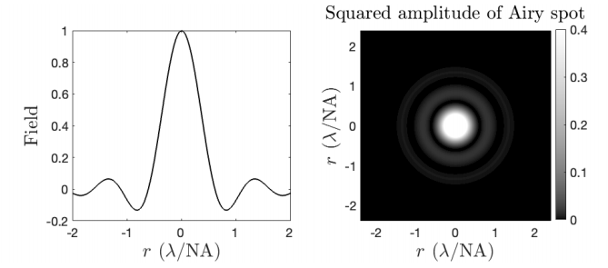
It seems that the diffraction model of light confirms what we know from geometrical optics. But in the previous two examples we discarded the influence of the finite size of the pupil, i.e. we have left out of consideration the function \(1_{\odot_{a}}\) in calculating the Fourier transform. If \(U_{0}(x, y)=1\) in the entrance pupil and we take the finite size of the pupil properly into account, the \(\delta\)-peaks become blurred: the focused field is then given by the Fourier transform of the circular disc with radius \(a\). evaluated at spatial frequencies \(\xi=\frac{x}{\lambda f}, \eta=\frac{y}{\lambda f}\). This field is called the Airy spot and is given by (See Appendix E.17): \[U(x, y, z)=\frac{\pi a^{2}}{\lambda f} \frac{2 J_{1}\left(2 \pi \frac{a}{\lambda f} \sqrt{x^{2}+y^{2}}\right)}{\frac{2 \pi a}{\lambda f} \sqrt{x^{2}+y^{2}}}, \quad \text { Airy pattern for focusing, } \nonumber \] where we have omitted the phase factors in front of the Fourier transform. The pattern is shown in Figure \(\PageIndex{1}\). It is circular symmetric and consists of a central maximum surrounded by concentric rings of alternating zeros and secondary maxima with rapidly decreasing amplitudes. In cross-section, as function of \(r=\sqrt{x^{2}+y^{2}}\), the Airy pattern is very similar (but not identical) to the sinc-function. From the uncertainty principle shown in Figure 6.5.3 it follows that the size of the focal spot decreases as \(a\) increases, and from ( \(\PageIndex{11}\) ) we see that the Airy function is a function of the dimensionless variable \(a r /(\lambda f)\). Hence the focal spot becomes narrower as \(a /(\lambda f)\) increases. The Numerical Aperture \((N A)\) is defined by \[\mathrm{NA}=\frac{a}{f}, \quad \text { numerical aperture. } \nonumber \]

Since the first zero of the Airy pattern occurs for \(2 \operatorname{ar} /(\lambda f)=1.22\), the size of the focal spot can be estimated as \[Size\space of\space focal\space spot ≈ 0.6\frac{\lambda}{NA} \nonumber \]

Figure \(\PageIndex{2}\): Left: cross section of the field of the Airy pattern. Right: intensity pattern of the Airy pattern.

6.8.2 Imaging by a lens

It follows from the derivations in the previous section that the Airy pattern is the image of a point source infinitely far in front of a lens. In this section we study the imaging of a general object. Consider first a point object at \(z=s_{o}<0\) in front of a lens with focal distance \(f>0\). The field in image space is derived similar to the focused field in the previous section. We postulate that the lens transforms the field radiated by the point object into a spherical wave in the exit pupil, which converges to the ideal image point of Gaussian geometrical optics. If we propagate this spherical field in the exit pupil to the image plane using the Fresnel diffraction integral, then for an object point on the optical axis we find the same Airy pattern as before and as shown in Figure \(\PageIndex{2}\), except that the variable \(a r /(\lambda f)\) must be replaced by \[\frac{a r}{\lambda s_{i}} \nonumber \] where \(s_{i}\) is the image position as given by the Lens Law. This field is called the Point Spread Function (PSF for short). Hence, \[\operatorname{PSF}(x, y)=\frac{\pi a^{2}}{\lambda s_{i}} \frac{J_{1}\left(2 \pi \frac{a}{\lambda s_{i}} \sqrt{x^{2}+y^{2}}\right)}{\frac{2 \pi a}{\lambda s_{i}} \sqrt{x^{2}+y^{2}}}, \quad \text { Airy pattern for imaging. } \nonumber \]

For object points that are not on the optical axis, the PSF is translated such that it is centred on the ideal Gaussian image point.

Usually we assume that we know the field transmitted or reflected by an object in the socalled object plane, which is the plane immediately behind the object (on the side of the lens). The object plane is discretised by a set of points and the images of these points are assumed to be given by translated versions of the PSF: \[\operatorname{PSF}\left(x-x_{i}, y-y_{i}\right) \nonumber \] where \(\left(x_{i}, y_{i}\right)\) are the transverse coordinates of the image point according to Gaussian geometrical optics.

The total image field is obtained by summing (integrating) over these PSFs, weighted by the field at the object points: \[U_{i}\left(x, y, s_{i}\right)=\iint \operatorname{PSF}\left(x-M x_{o}, x-M y_{o}\right) U_{o}\left(x_{o}, y_{o}, s_{o}\right) \mathrm{d} x_{o} \mathrm{~d} y_{o} . \nonumber \] where \(x_{o}=x_{i} / M, y_{o}=y_{i} / M\) is the image point and \(M\) is the magnification. If the magnification is unity, the image field is a convolution between the PSF and the object field. If the magnification differs from unity, the integral can be made into a convolution by rescaling the coordinates in image space.

It is clear from \(\PageIndex{15}\) that larger radius \(a\) of the lens and smaller wavelength \(\lambda\) imply a narrower PSF. This in turn implies that the kernel in the convolution is more sharply peaked and hence that the resolution of the image is higher.

Remarks

1. If laser light is used to illuminate the object, the object field may in general be considered to be perfectly coherent. This implies that a detector in the image plane would measure the squared modulus of the complex field ( \(\PageIndex{16}\)): \[I_{i}\left(x, y, s_{i}\right)=\left|\iint \operatorname{PSF}\left(x-M x_{o}, y-M y_{o}\right) U_{o}\left(x_{o}, y_{o}, s_{o}\right) \mathrm{d} x_{o} \mathrm{~d} y_{o}\right|^{2} . \nonumber \]

In this case the system is called a coherent imaging system.

2. If the object is an spatially completely incoherent source, the images of the point sources of which the source (object) consists cannot interfere in the image plane. Therefore, in this case the intensity in the image plane is given by the incoherent sum: \[I_{i}\left(x, y, s_{i}\right)=\iint\left|\operatorname{PSF}\left(x-M x_{o}, y-M x_{o}\right)\right|^{2} I_{o}\left(x_{o}, y_{o}, s_{o}\right) \mathrm{d} x_{o} \mathrm{~d} y_{o}, \nonumber \] where \(I_{o}=\left|U_{o}\right|^{2}\) is the intensity of the object. Hence the image intensity is expressed in the intensity of the object by a convolution with the intensity of the PSF. This system is called a incoherent imaging system.

3. An object is often illuminated by a spatially incoherent light source and then imaged. The field reflected or transmitted by the object is then partially coherent. We have shown in Chapter 5 that the degree of mutual coherence in the object increases when the distance between the source and the object is increased. The detected intensity in the image plane can be computed by splitting up the spatially incoherent source into sufficiently many mutually incoherent point sources and considering the fields in the image plane due to the illumination by each individual point source. The total intensity in the image plane is then the sum of the individual intensities.

6.8.3 Spatial Light Modulators and Optical Fourier Filtering

• SLM. The field in the entrance pupil of a lens can be changed spatially by a so-called spatial light modulator (SLM). A SLM has thousands of pixels by which very general fields can be made. By applying three SLMs in series, one can tune the polarisation, the phase and the amplitude pixel by pixel and hence very desired pupil fields can be realised which after focusing, can give very special focused fields. An example is an electric field with only a longitudinal component (i.e. only a \(E_{z}\)-component) in the focal point.
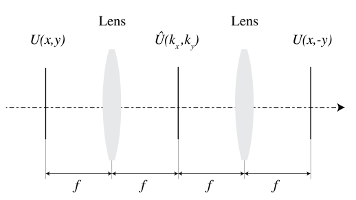
• Fourier filtering. Suppose we have the setup as shown in Figure \(\PageIndex{3}\). With one lens we can create the Fourier transform of some field \(U(x, y)\). If a mask is put in the focal plane and a second lens is used to refocus the light, the inverse Fourier transform of the field after the mask is obtained. This procedure is called Fourier filtering using lenses. Fourier filtering means that the amplitude and/or phase of the plane waves in the angular spectrum of the field are manipulated. An application of this idea is the phase contrast microscope.

Figure \(\PageIndex{3}\): Set-up for Fourier filtering. The first lens creates a Fourier transform of \(U(x, y)\), to which we can apply some operation (e.g. applying different phase shifts to different parts of the field). The second lens then applies another Fourier transform (which is the same as the inverse Fourier transform and a mirror transformation).