4.2: Spherical Aberration
- Page ID
- 7088

\( \newcommand{\vecs}[1]{\overset { \scriptstyle \rightharpoonup} {\mathbf{#1}} } \)
\( \newcommand{\vecd}[1]{\overset{-\!-\!\rightharpoonup}{\vphantom{a}\smash {#1}}} \)
\( \newcommand{\dsum}{\displaystyle\sum\limits} \)
\( \newcommand{\dint}{\displaystyle\int\limits} \)
\( \newcommand{\dlim}{\displaystyle\lim\limits} \)
\( \newcommand{\id}{\mathrm{id}}\) \( \newcommand{\Span}{\mathrm{span}}\)
( \newcommand{\kernel}{\mathrm{null}\,}\) \( \newcommand{\range}{\mathrm{range}\,}\)
\( \newcommand{\RealPart}{\mathrm{Re}}\) \( \newcommand{\ImaginaryPart}{\mathrm{Im}}\)
\( \newcommand{\Argument}{\mathrm{Arg}}\) \( \newcommand{\norm}[1]{\| #1 \|}\)
\( \newcommand{\inner}[2]{\langle #1, #2 \rangle}\)
\( \newcommand{\Span}{\mathrm{span}}\)
\( \newcommand{\id}{\mathrm{id}}\)
\( \newcommand{\Span}{\mathrm{span}}\)
\( \newcommand{\kernel}{\mathrm{null}\,}\)
\( \newcommand{\range}{\mathrm{range}\,}\)
\( \newcommand{\RealPart}{\mathrm{Re}}\)
\( \newcommand{\ImaginaryPart}{\mathrm{Im}}\)
\( \newcommand{\Argument}{\mathrm{Arg}}\)
\( \newcommand{\norm}[1]{\| #1 \|}\)
\( \newcommand{\inner}[2]{\langle #1, #2 \rangle}\)
\( \newcommand{\Span}{\mathrm{span}}\) \( \newcommand{\AA}{\unicode[.8,0]{x212B}}\)
\( \newcommand{\vectorA}[1]{\vec{#1}} % arrow\)
\( \newcommand{\vectorAt}[1]{\vec{\text{#1}}} % arrow\)
\( \newcommand{\vectorB}[1]{\overset { \scriptstyle \rightharpoonup} {\mathbf{#1}} } \)
\( \newcommand{\vectorC}[1]{\textbf{#1}} \)
\( \newcommand{\vectorD}[1]{\overrightarrow{#1}} \)
\( \newcommand{\vectorDt}[1]{\overrightarrow{\text{#1}}} \)
\( \newcommand{\vectE}[1]{\overset{-\!-\!\rightharpoonup}{\vphantom{a}\smash{\mathbf {#1}}}} \)
\( \newcommand{\vecs}[1]{\overset { \scriptstyle \rightharpoonup} {\mathbf{#1}} } \)
\(\newcommand{\longvect}{\overrightarrow}\)
\( \newcommand{\vecd}[1]{\overset{-\!-\!\rightharpoonup}{\vphantom{a}\smash {#1}}} \)
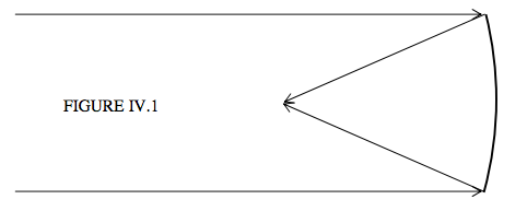
\(\newcommand{\avec}{\mathbf a}\) \(\newcommand{\bvec}{\mathbf b}\) \(\newcommand{\cvec}{\mathbf c}\) \(\newcommand{\dvec}{\mathbf d}\) \(\newcommand{\dtil}{\widetilde{\mathbf d}}\) \(\newcommand{\evec}{\mathbf e}\) \(\newcommand{\fvec}{\mathbf f}\) \(\newcommand{\nvec}{\mathbf n}\) \(\newcommand{\pvec}{\mathbf p}\) \(\newcommand{\qvec}{\mathbf q}\) \(\newcommand{\svec}{\mathbf s}\) \(\newcommand{\tvec}{\mathbf t}\) \(\newcommand{\uvec}{\mathbf u}\) \(\newcommand{\vvec}{\mathbf v}\) \(\newcommand{\wvec}{\mathbf w}\) \(\newcommand{\xvec}{\mathbf x}\) \(\newcommand{\yvec}{\mathbf y}\) \(\newcommand{\zvec}{\mathbf z}\) \(\newcommand{\rvec}{\mathbf r}\) \(\newcommand{\mvec}{\mathbf m}\) \(\newcommand{\zerovec}{\mathbf 0}\) \(\newcommand{\onevec}{\mathbf 1}\) \(\newcommand{\real}{\mathbb R}\) \(\newcommand{\twovec}[2]{\left[\begin{array}{r}#1 \\ #2 \end{array}\right]}\) \(\newcommand{\ctwovec}[2]{\left[\begin{array}{c}#1 \\ #2 \end{array}\right]}\) \(\newcommand{\threevec}[3]{\left[\begin{array}{r}#1 \\ #2 \\ #3 \end{array}\right]}\) \(\newcommand{\cthreevec}[3]{\left[\begin{array}{c}#1 \\ #2 \\ #3 \end{array}\right]}\) \(\newcommand{\fourvec}[4]{\left[\begin{array}{r}#1 \\ #2 \\ #3 \\ #4 \end{array}\right]}\) \(\newcommand{\cfourvec}[4]{\left[\begin{array}{c}#1 \\ #2 \\ #3 \\ #4 \end{array}\right]}\) \(\newcommand{\fivevec}[5]{\left[\begin{array}{r}#1 \\ #2 \\ #3 \\ #4 \\ #5 \\ \end{array}\right]}\) \(\newcommand{\cfivevec}[5]{\left[\begin{array}{c}#1 \\ #2 \\ #3 \\ #4 \\ #5 \\ \end{array}\right]}\) \(\newcommand{\mattwo}[4]{\left[\begin{array}{rr}#1 \amp #2 \\ #3 \amp #4 \\ \end{array}\right]}\) \(\newcommand{\laspan}[1]{\text{Span}\{#1\}}\) \(\newcommand{\bcal}{\cal B}\) \(\newcommand{\ccal}{\cal C}\) \(\newcommand{\scal}{\cal S}\) \(\newcommand{\wcal}{\cal W}\) \(\newcommand{\ecal}{\cal E}\) \(\newcommand{\coords}[2]{\left\{#1\right\}_{#2}}\) \(\newcommand{\gray}[1]{\color{gray}{#1}}\) \(\newcommand{\lgray}[1]{\color{lightgray}{#1}}\) \(\newcommand{\rank}{\operatorname{rank}}\) \(\newcommand{\row}{\text{Row}}\) \(\newcommand{\col}{\text{Col}}\) \(\renewcommand{\row}{\text{Row}}\) \(\newcommand{\nul}{\text{Nul}}\) \(\newcommand{\var}{\text{Var}}\) \(\newcommand{\corr}{\text{corr}}\) \(\newcommand{\len}[1]{\left|#1\right|}\) \(\newcommand{\bbar}{\overline{\bvec}}\) \(\newcommand{\bhat}{\widehat{\bvec}}\) \(\newcommand{\bperp}{\bvec^\perp}\) \(\newcommand{\xhat}{\widehat{\xvec}}\) \(\newcommand{\vhat}{\widehat{\vvec}}\) \(\newcommand{\uhat}{\widehat{\uvec}}\) \(\newcommand{\what}{\widehat{\wvec}}\) \(\newcommand{\Sighat}{\widehat{\Sigma}}\) \(\newcommand{\lt}{<}\) \(\newcommand{\gt}{>}\) \(\newcommand{\amp}{&}\) \(\definecolor{fillinmathshade}{gray}{0.9}\)We’ll begin by looking at the spherical aberration resulting from reflection from a spherical mirror. We have hitherto assumed that a parallel beam of light, after reflection from a spherical mirror, comes to a focus at a point, and that the distance of the focal point from the surface of the mirror is half the radius of curvature of the mirror, as in Figure IV.1:
This is approximately true for a small aperture mirror (“aperture” meaning the ratio of the diameter to the focal length). This is not the case, however, for a large aperture mirror. In Figure IV.2 I have drawn a hemispherical mirror. I assume that there is an incident beam of light (not drawn) coming in horizontally from the left, and I have drawn the rays after reflection from the mirror. (Some of the rays will be reflected a second time from the surface before eventually escaping, but I have not drawn the rays after a second reflection because they would only clutter up the diagram and are not pertinent in describing what I want to describe. You can see that the reflected rays are bounded by an envelope known as a caustic curve, shown as a dashed red curve in Figure IV.2.
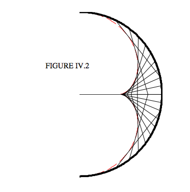
Can we find the equation to this caustic curve?
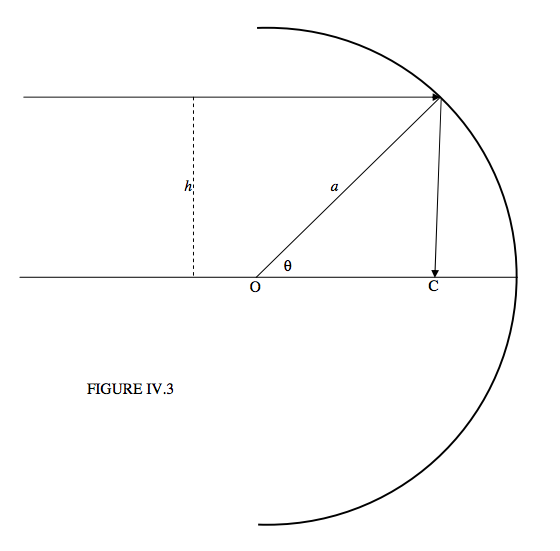
We’ll take the centre of curvature of the mirror as origin O of coordinates, and suppose that the radius of curvature of the mirror is \(a\). Let us consider the adventures of a ray of light coming in parallel to the horizontal \((x)\) axis and at a height \(h\) from it. The equation to the incoming light ray is just \(y = h\), and the equation to the mirror surface is \( x^2+y^2=a^2\). A little bit of coordinate geometry will enable us to determine that the equation to the reflected ray is
\[y = \frac{h}{a^2-2h^2}\left[\left(2 \sqrt{a^2-h^2}x-a^2\right)\right], \label{eq:4.2.1} \]
and that it crosses the \(x\)-axis at a point C such that
\[OC = \frac{a^2}{2\sqrt{a^2-h^2}}. \label{eq:4.2.2} \]
It is also convenient to write these formulas in terms of the angle \(\theta\), which is given by \(h = a\sin \theta\). After a little algebra and application of some trigonometric identities, we obtain
\[ y = x \tan 2 \theta - \frac{a\sin\theta}{\cos2\theta}\label{eq:4.2.3} \]
for the equation to the reflected ray, and
\[ OC = \frac{1}{2} a \sec \theta. \label{eq:4.2.4} \]
We can write Equation \(\ref{eq:4.2.3}\) as
\[ f(x,y;\theta)= x\tan2\theta-\frac{a\sin\theta}{\cos2\theta}-y=0.\label{eq:4.2.5} \]
From our long-forgotten, yellowed and mildewy mathematics notes, we recall that to find the equation to the envelope of a family of curves of the form \(f(x,y;\theta)=0\), we have to eliminate the parameter \(\theta\) from that equation and the equation \(\frac{\partial f}{\partial \theta}=0\). After some more algebra and more application of trigonometric identities, we find that the latter equation comes to
\[ x=a\cos\theta.(\frac{3}{2}-\cos^2\theta).\label{eq:4.2.6} \]
So, all we have to do is to eliminate the parameter \(\theta\) from Equations \(\ref{eq:4.2.3}\) and \(\ref{eq:4.2.6}\), and this would give us the \(x , y\) equation to the caustic curve. These two equations are, in fact, the parametric equations to the caustic curve. Now I don’t know how easy it would be to eliminate \(\theta\). Since Equation \(\ref{eq:4.2.6}\) is a cubic equation in \(\cos \theta\), I suspect that it might not be particularly easy. But (as is often the case with two parametric equations to a curve) we can happily plot the curve numerically, without having to eliminate the parameter algebraically. Thus, in order to plot the red curve in Figure IV.2, I varied \(\theta\) from −90° to +90°, and calculated \(x\) from Equation \(\ref{eq:4.2.6}\), and I then calculated \(y\) from Equation \(\ref{eq:4.2.3}\).
To avoid spherical aberration, telescope mirrors can be made in a paraboloidal shape. It can be shown that an incident beam of light, coming in parallel to the axis of a paraboloidal mirror, after reflection will come to single focal point, namely at the focus of the parabola. A proof of this is given in Section 2.4 of Chapter 2 of my Celestial Mechanics notes and is not repeated there. In that Chapter, it is also shown that, if a bucket of liquid is rotated about a vertical axis, the surface of the liquid will take up a paraboloidal shape, and mention is made there of two applications to the manufacture of paraboloidal mirrors. In one, a vat of molten glass is rotated, and is gradually cooled down until the glass solidifies into a paraboloidal shape. In the other, a container of mercury is rotated, the surface of the mercury taking up a paraboloidal shape, and this liquid paraboloid is then used as the main mirror of a reflecting telescope. While it can observe only close to the zenith, some excellent results have been obtained. I shan’t repeat it here, but you might want to refer to the above-mentioned notes, since it is pertinent here.
This property (of light being reflected from the surface of a parabola to a single focal point) applies only to light coming in parallel to the axis of the paraboloid. Consequently paraboloidal telescope mirrors have only a rather narrow field of view. A Schmidt telescope uses a spherical mirror (hence a large field of view) and, to avoid spherical aberration, a corrector plate is mounted in front of the mirror. Typically the spherical mirror is at the “bottom end” of the telescope tube, and the corrector plate is at the “top end”. The corrector plate causes light that is coming in parallel to the telescope tube, but some distance from the axis of the tube, to diverge slightly from the axis before reaching the spherical mirror. In this manner all of the incoming light, after reflection from the mirror, comes to a focus at a single point.
A lens also suffers from spherical aberration, of course, but it does not lend itself to such simple analysis as for a spherical mirror. One needs to perform detailed numerical ray-tracing to find the exact shape of the caustic curve for a lens. We showed, however, in Section 1.4 of Chapter 1, that refraction even at a plane surface produces spherical aberration.
One might wonder, given that a paraboloidal mirror when used on axis is free of spherical aberration, whether a lens made with paraboloidal surfaces, is also free of spherical aberration. Alas, that is not so.
One can, however, design a lens with spherical surfaces that minimize the spherical aberration, by suitable choice of the radii or curvature of the lens surfaces. This is called “bending the lens”.
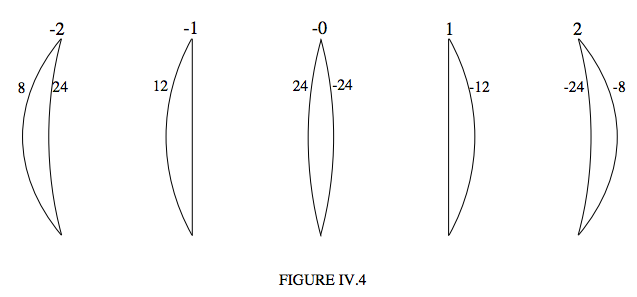
For example, Figure IV.4 shows five lenses, in which I have written, beside each surface, its radius of curvature in cm. In what follows I assume that the lens is “thin” in the sense that its thickness is very small compared with any other distances under discussion. If the refractive index is 1.6, each of these lenses has a focal length of 20 cm.
You can characterize the shape of a lens by means of its shape factor.
\[ q=\frac{r_1+r_2}{r_1-r_2}\label{eq:4.2.7} \]
In Figure IV.4 I have written the shape factor above each lens.
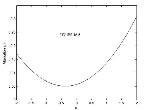
For light coming in horizontally near the axis, the focal length of each of these lenses is 20 cm. However, light coming in horizontally at some distance from the axis, after passage through the lens, falls a little short of 20 cm. We may characterize the spherical aberration by the amount it falls short. Assuming that the lenses are thin (compared with any other distances under consideration) I calculated the shortfall for a ray of light coming in from the left at a height of 1 cm from the axis. This is shown in Figure IV.5, in which I have drawn the shortfall (labelled “Aberration” in the figure) versus shape factor \(q\). It is seen that the aberration is least for a shape factor of about \(q = −0.38\). The radii of curvatures of the lens must satisfy equation \(\ref{eq:4.2.7}\) as well as \(q = −0.38\)
\[\frac{1}{f}=(n-1)\left(\frac{1}{r_1}-\frac{1}{r_2}\right), \label{eq:4.2.8} \]
so that, for \(f\) = 20 cm and \(q\) = −0.38, the radii of curvature for least spherical aberration should be \(r_1\) = 17.4 cm and \(r_2\) = −38.7 cm.
Of course, you have to use the lens the right way round! If you turn it round, or if light is coming in from the right, the shape factor is +0.38, and the spherical aberration is not at a minimum. Mind you, the minimum is fairly shallow, so you can vary the shape factor a fair amount without grossly increasing the spherical aberration.