7.2: Spin

For orbital angular momentum we found that \(2 l+1\) must be an integer, and moreover the spatial properties of the wave function force \(l\) to be an integer as well. However, we can also construct states with half-integer \(l\), but this must then be an internal degree of freedom. This is called spin angular momentum, or spin for short. We will show later in the course that the spin observable is interpreted as an intrinsic magnetic moment of a system.

To describe spin, we switch from L to S, which is no longer related to r and p. The commutation relations between the components \(S_{i}\) are the same as for \(L_{i}\),

\[\left[S_{i}, S_{j}\right]=i \hbar \epsilon_{i j k} S_{k}\tag{7.24}\]

so S and L obey the same algebra. The commutation relations between S and L, r, and p vanish:

\[\left[S_{i}, L_{j}\right]=\left[S_{i}, r_{j}\right]=\left[S_{i}, p_{j}\right]=0.\tag{7.25}\]

Therefore, spin generates a whole new vector space, since it commutes with observables that themselves do not commute (like \(r_{j}\) and \(p_{j}\)), and it is independent of the spatial degrees of freedom.

Since the commutation relations for S (its algebra) are the same as for L, we can immediately copy the algebraic structure of the eigenstates and eigenvalues:

\[\begin{aligned}
&S_{z}\left|s, m_{s}\right\rangle=m_{s} \hbar\left|s, m_{s}\right\rangle, \quad \text { with } s=0, \frac{1}{2}, 1, \frac{3}{2}, 2, \ldots \\
&\mathbf{S}^{2}\left|s, m_{s}\right\rangle=s(s+1) \hbar^{2}\left|s, m_{s}\right\rangle.
\end{aligned}\tag{7.26}\]

When \(s=\frac{1}{2}\), the system has two levels (a qubit) with spin eigenstates \(\left|\frac{1}{2}, \frac{1}{2}\right\rangle\) and \(\left|\frac{1}{2},-\frac{1}{2}\right\rangle\). We often write \(m_{s}=+\frac{1}{2}=\uparrow\) (“up”) and \(m_{s}=-\frac{1}{2}=\downarrow\) (“down”), which finds its origin in the measurement outcomes of electron spin in a Stern-Gerlach apparatus.

Now that we have introduced a whole new vector space related to spin, how do we write the wave function of a particle with spin? Without spin, the wave function is a normal single-valued function \(\psi(\mathbf{r}, t)=\langle\mathbf{r} \mid \psi(t)\rangle\) of space and time coordinates. Now we have to add the spin degree of freedom. For each spin \(\left(\uparrow \text { or } \downarrow \text { when } s=\frac{1}{2}\right)\), we have a wave function \(\psi_{\uparrow}(\mathbf{r}, t)\) for the particle with spin up, and \(\psi_{\downarrow}(\mathbf{r}, t)\) for the particle with spin down. We can write this as a vector:

\[\psi(\mathbf{r}, t)=\left(\begin{array}{l}
\psi_{\uparrow}(\mathbf{r}, t) \\
\psi_{\downarrow}(\mathbf{r}, t)
\end{array}\right).\tag{7.27}\]

The spin degree of freedom generates a vector space, after all. The vector \(\psi\) is called a spinor.

Expectation values are evaluated in the usual way, but now we have to sum over the spin degree of freedom, as well as integrate over space. For example, the probability of finding a particle with spin up in a region \(\Omega\) of space is given by

\[p(\uparrow, \Omega)=\sum_{m_{s}=\uparrow, \downarrow} \int_{\Omega} d \mathbf{r} \delta_{m_{s}, \uparrow}\left|\psi_{m_{s}}(\mathbf{r}, t)\right|^{2}=\int_{\Omega} d \mathbf{r}\left|\psi_{\uparrow}(\mathbf{r}, t)\right|^{2},\tag{7,28}\]

and the expectation value of finding a particle with any spin in a region \(\Omega\) of space is given by

\[p(\Omega)=\sum_{m_{s}=\uparrow, \downarrow} \int_{\Omega} d \mathbf{r}\left|\psi_{m_{s}}(\mathbf{r}, t)\right|^{2}.\tag{7.29}\]

The normalization of the spinor is such that

\[\sum_{m_{s}=\uparrow, \downarrow} \int_{V} d \mathbf{r}\left|\psi_{m_{s}}(\mathbf{r}, t)\right|^{2}=1,\tag{7.30}\]

where \(V\) is the entire space available to the particle (this may be the entire universe, or the volume of a box with impenetrable walls, etc.).

If spin is represented by \((2 s+1)\)-dimensional spinors (vectors), then spin transformations (operators) are represented by \((2 s+1) \times(2 s+1)\) matrices. In the two-dimensional case, we have by construction:

\[S_{z}|\uparrow\rangle=\frac{\hbar}{2}\left(\begin{array}{l} 1 \\ 0
\end{array}\right) \quad \text { and } \quad S_{z}|\downarrow\rangle=-\frac{\hbar}{2}\left(\begin{array}{l} 0 \\ 1 \end{array}\right),\tag{7.31}\]

which means that the matrix representation of \(S_{z}\) is given by

\[S_{z}=\frac{\hbar}{2}\left(\begin{array}{cc}
1 & 0 \\
0 & -1
\end{array}\right).\tag{7.32}\]

Next, the ladder operators act according to

\[S_{+}|\uparrow\rangle=0, \quad S_{+}|\downarrow\rangle=\hbar|\uparrow\rangle, \quad S_{-}|\uparrow\rangle=\hbar|\downarrow\rangle, \quad S_{-}|\downarrow\rangle=0,\tag{7.33}\]

which leads to the matrix representation

\[S_{+}=\hbar\left(\begin{array}{ll} 0 & 1 \\ 0 & 0
\end{array}\right) \quad \text { and } \quad S_{-}=\hbar\left(\begin{array}{ll} 0 & 0 \\ 1 & 0 \end{array}\right).\tag{7.34}\]

From \(S_{\pm}=S_{x} \pm i S_{y}\) we can then deduce that

\[S_{x}=\frac{\hbar}{2}\left(\begin{array}{ll} 0 & 1 \\ 1 & 0
\end{array}\right) \quad \text { and } \quad S_{y}=\frac{\hbar}{2}\left(\begin{array}{cc} 0 & -i \\ i & 0 \end{array}\right).\tag{7.35}\]

We often define \(S_{i} \equiv \frac{1}{2} \hbar \sigma_{i}\), where \(\sigma_{i}\) are the so-called Pauli matrices. Previously, we have called these matrices \(X\), \(Y\), and \(Z\). The commutation relations of the Pauli matrices are

\[\left[\sigma_{i}, \sigma_{j}\right]=2 i \epsilon_{i j k} \sigma_{k} \quad \text { or } \quad\left[\frac{\sigma_{i}}{2}, \frac{\sigma_{j}}{2}\right]=i \epsilon_{i j k} \frac{\sigma_{k}}{2}.\tag{7.36}\]

Other important properties of the Pauli matrices are

\[\left\{\sigma_{i}, \sigma_{j}\right\} \equiv \sigma_{i} \sigma_{j}+\sigma_{j} \sigma_{i}=2 \delta_{i j} \mathbb{I} \quad \text { (anti-commutator). }\tag{7.37}\]

They are both Hermitian and unitary, and the square of the Pauli matrices is the identity: \(\sigma_{i}^{2}=\mathbb{I}\). Moreover, they obey an “orthogonality” relation

\[\frac{1}{2} \operatorname{Tr}\left(\sigma_{i} \sigma_{j}\right)=\delta_{i j}.\tag{7.38}\]

The proof of this statement is as follows:

\[\sigma_{i} \sigma_{j}=\sigma_{i} \sigma_{j}+\sigma_{j} \sigma_{i}-\sigma_{j} \sigma_{i}=\left\{\sigma_{i}, \sigma_{j}\right\}-\sigma_{j} \sigma_{i}=2 \delta_{i j}^{\mathbb{I}}-\sigma_{j} \sigma_{i}.\tag{7.39}\]

Taking the trace then yields

\[\operatorname{Tr}\left(2 \delta_{i j} \mathbb{I}-\sigma_{j} \sigma_{i}\right)=\operatorname{Tr}\left(\sigma_{i} \sigma_{j}\right)=\operatorname{Tr}\left(\sigma_{j} \sigma_{i}\right),\tag{7.40}\]

or (using \(\operatorname{Tr}(\mathbb{I})=2\))

\[2 \operatorname{Tr}\left(\sigma_{j} \sigma_{i}\right)=4 \delta_{i j},\tag{7.41}\]

which proves Eq. (7.38). If we define \(\sigma_{0} \equiv \mathbb{I}\), we can extend this proof to the four-dimensional case

\[\frac{1}{2} \operatorname{Tr}\left(\sigma_{\mu} \sigma_{v}\right)=\delta_{\mu v}\tag{7.42}\]

with \(\mu, v=0,1,2,3\).

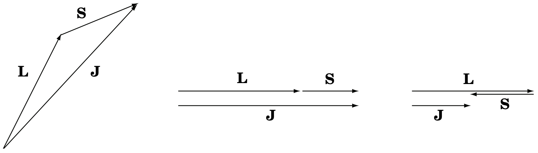Figure 3: Addition of angular momentum.

We can then write any 2×2 matrix as a sum over the two-dimensional Pauli operators:

\[A=\sum_{\mu} a_{\mu} \sigma_{\mu},\tag{7.43}\]

since

\(\frac{1}{2} \operatorname{Tr}\left(A \sigma_{v}\right)=\frac{1}{2} \operatorname{Tr}\left(\sum_{\mu} a_{\mu} \sigma_{\mu} \sigma_{v}\right)=\frac{1}{2} \sum_{\mu} a_{\mu} \operatorname{Tr}\left(\sigma_{\mu} \sigma_{v}\right)=\sum_{\mu} a_{\mu} \delta_{\mu v}=a_{v}\tag{7.44}\]

The Pauli matrices and the identity matrix form a basis for the 2×2 matrices, and we can write

\[A=a_{0} \mathbb{I}+\mathbf{a} \cdot \sigma=\left(\begin{array}{cc}
a_{0}+a_{z} & a_{x}-i a_{y} \\
a_{x}+i a_{y} & a_{0}-a_{z}
\end{array}\right)\tag{7.45}\]

where we used the notation \(\boldsymbol{\sigma}=\left(\sigma_{x}, \sigma_{y}, \sigma_{z}\right)\).