
2.11: Evolution of Wave-Packets
( \newcommand{\kernel}{\mathrm{null}\,}\)
We have seen, in Equation ([e2.45]), how to write the wavefunction of a particle that is initially localized in x-space. Let us examine how this wavefunction evolves in time. According to Equation ([e2.42]), we have ψ(x,t)=∫∞−∞ˉψ(k)eiϕ(k)dk, where ϕ(k)=kx−ω(k)t. The function ˉψ(k) is obtained by Fourier transforming the wavefunction at t=0. [See Equations ([e2.42a]) and ([e2.51]).] According to Equation ([e2.53]), |ˉψ(k)| is strongly peaked around k=k0. Thus, it is a reasonable approximation to Taylor expand ϕ(k) about k0. Keeping terms up to second order in k−k0, we obtain ψ(x,t)∝∫∞−∞ˉψ(k)exp[i{ϕ0+ϕ′0(k−k0)+12ϕ″0(k−k0)2}], where ϕ0=ϕ(k0)=k0x−ω0t,ϕ′0=dϕ(k0)dk=x−vgt,ϕ″0=d2ϕ(k0)dk2=−αt, with ω0=ω(k0),vg=dω(k0)dk,α=d2ω(k0)dk2. Substituting from Equation ([e2.51]), rearranging, and then changing the variable of integration to y=(k−k0)/(2Δk), we get ψ(x,t)∝ei(k0x−ω0t)∫∞−∞eiβ1y−(1+iβ2)y2dy, where β1=2Δk(x−x0−vgt),β2=2α(Δk)2t. Incidentally, Δk=1/(2Δx), where Δx is the initial width of the wave-packet. The previous expression can be rearranged to give ψ(x,t)∝ei(k0x−ω0t)−(1+iβ2)β2/4∫∞−∞e−(1+iβ2)(y−y0)2dy, where y0=iβ/2 and β=β1/(1+iβ2). Again changing the variable of integration to z=(1+iβ2)1/2(y−y0), we get ψ(x,t)∝(1+iβ2)−1/2ei(k0x−ω0t)−(1+iβ2)β2/4∫∞−∞e−z2dz. The integral now just reduces to a number. Hence, we obtain ψ(x,t)∝exp[i(k0x−ω0t)−(x−x0−vgt)2{1−i2α(Δk)2t}/(4σ2)][1+i2α(Δk)2t]1/2, where σ2(t)=(Δx)2+α2t24(Δx)2. Note that the previous wavefunction is identical to our original wavefunction ([e2.45]) at t=0. This justifies the approximation that we made earlier by Taylor expanding the phase factor ϕ(k) about k=k0.
According to Equation ([exxx]), the probability density of our particle as a function of time is written |ψ(x,t)|2∝σ−1(t)exp[−(x−x0−vgt)22σ2(t)]. Hence, the probability distribution is a Gaussian, of characteristic width σ(t), that peaks at x=x0+vgt. The most likely position of our particle coincides with the peak of the distribution function. Thus, the particle’s most likely position is given by x=x0+vgt. It can be seen that the particle effectively moves at the uniform velocity vg=dωdk, which is known as the group-velocity. In other words, a plane-wave travels at the phase-velocity, vp=ω/k, whereas a wave-packet travels at the group-velocity, vg=dω/dt. It follows from the dispersion relation ([e2.38]) for particle waves that vg=pm. However, it can be seen from Equation ([e2.31]) that this is identical to the classical particle velocity. Hence, the dispersion relation ([e2.38]) turns out to be consistent with classical physics, after all, as soon as we realize that individual particles must be identified with wave-packets rather than plane-waves. In fact, a plane-wave is usually interpreted as a continuous stream of particles propagating in the same direction as the wave.
According to Equation ([e2.70]), the width of our wave-packet grows as time progresses. Indeed, it follows from Equations ([e2.38]) and ([e2.64]) that the characteristic time for a wave-packet of original width Δx to double in spatial extent is t2∼m(Δx)2ℏ. For instance, if an electron is originally localized in a region of atomic scale (i.e., Δx∼10−10m) then the doubling time is only about 10−16s. Evidently, particle wave-packets (for freely-moving particles) spread very rapidly.
Note, from the previous analysis, that the rate of spreading of a wave-packet is ultimately governed by the second derivative of ω(k) with respect to k. [See Equations ([e2.64]) and ([e2.70]).] This explains why a functional relationship between ω and k is generally known as a dispersion relation—it governs how fast wave-packets disperse as time progresses. However, for the special case where ω is a linear function of k, the second derivative of ω with respect to k is zero, and, hence, there is no dispersion of wave-packets: that is, wave-packets propagate without changing shape. The dispersion relation ([e2.7]) for light-waves is linear in k. It follows that light pulses propagate through a vacuum without spreading. Another property of linear dispersion relations is that the phase-velocity, vp=ω/k, and the group-velocity, vg=dω/dk, are identical. Thus, plane light-waves and light pulses both propagate through a vacuum at the characteristic speed c=3×10⁸m/s. Of course, the dispersion relation ([e2.38]) for particle waves is not linear in k. Hence, particle plane-waves and particle wave-packets propagate at different velocities, and particle wave-packets also gradually disperse as time progresses.
Heisenberg’s Uncertainty Principle
According to the analysis contained in the previous two sections, a particle wave-packet that is initially localized in x-space with characteristic width Δx is also localized in k-space with characteristic width Δk=1/(2Δx). However, as time progresses, the width of the wave-packet in x-space increases, while that of the wave-packet in k-space stays the same. [After all, our previous analysis obtained ψ(x,t) from Equation ([e2.56]), but assumed that ˉψ(k) was given by Equation ([e2.51]) at all times.] Hence, in general, we can say that ΔxΔk≳ Furthermore, we can think of {\mit\Delta}x and {\mit\Delta} k as characterizing our uncertainty regarding the values of the particle’s position and wavenumber, respectively.
A measurement of a particle’s wavenumber, k, is equivalent to a measurement of its momentum, p, because p=\hbar \,k. Hence, an uncertainty in k of order {\mit\Delta} k translates to an uncertainty in p of order {\mit\Delta}p=\hbar\,{\mit\Delta}k. It follows from the previous inequality that \begin{equation}\Delta x \Delta p \gtrsim \frac{\hbar}{2}\end{equation} This is the famous Heisenberg uncertainty principle, first proposed by Werner Heisenberg in 1927 . According to this principle, it is impossible to simultaneously measure the position and momentum of a particle (exactly). Indeed, a good knowledge of the particle’s position implies a poor knowledge of its momentum, and vice versa. Note that the uncertainty principle is a direct consequence of representing particles as waves.
It can be seen from Equations ([e2.38]), ([e2.64]), and ([e2.70]) that, at large t, a particle wavefunction of original width {\mit\Delta} x (at t=0) spreads out such that its spatial extent becomes \label{espread} \sigma\sim \frac{\hbar\,t}{m\,{\mit\Delta}x}. It is easily demonstrated that this spreading is a consequence of the uncertainty principle. Because the initial uncertainty in the particle’s position is {\mit\Delta}x, it follows that the uncertainty in its momentum is of order \hbar/{\mit\Delta}x. This translates to an uncertainty in velocity of {\mit\Delta}v = \hbar/(m\,{\mit\Delta}x). Thus, if we imagine that parts of the wavefunction propagate at v_0+ {\mit\Delta}v/2, and others at v_0-{\mit\Delta}v/2, where v_0 is the mean propagation velocity, then the wavefunction will spread as time progresses. Indeed, at large t, we expect the width of the wavefunction to be \sigma \sim {\mit\Delta}v\,t \sim \frac{\hbar\,t}{m\,{\mit\Delta}x}, which is identical to Equation ([espread]). Evidently, the spreading of a particle wavefunction must be interpreted as an increase in our uncertainty regarding the particle’s position, rather than an increase in the spatial extent of the particle itself.
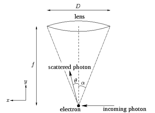
Figure 8: Heisenberg's microscope.
Figure [fh] illustrates a famous thought experiment known as Heisenberg’s microscope. Suppose that we try to image an electron using a simple optical system in which the objective lens is of diameter D and focal-length f. (In practice, this would only be possible using extremely short-wavelength light.) It is a well-known result in optics that such a system has a minimum angular resolving power of \lambda/D, where \lambda is the wavelength of the light illuminating the electron . If the electron is placed at the focus of the lens, which is where the minimum resolving power is achieved, then this translates to a uncertainty in the electron’s transverse position of {\mit\Delta}x \simeq f\,\frac{\lambda}{D}. However, \tan\alpha = \frac{D/2}{f}, where \alpha is the half-angle subtended by the lens at the electron. Assuming that \alpha is small, we can write \alpha\simeq \frac{D}{2\,f}, so {\mit\Delta} x\simeq \frac{\lambda}{2\,\alpha}. It follows that we can reduce the uncertainty in the electron’s position by minimizing the ratio \lambda/\alpha: that is, by employing short-wavelength radiation, and a wide-angle lens.
Let us now examine Heisenberg’s microscope from a quantum-mechanical point of view. According to quantum mechanics, the electron is imaged when it scatters an incoming photon towards the objective lens. Let the wavevector of the incoming photon have the (x,y) components (k,0). See Figure [fh]. If the scattered photon subtends an angle \theta with the center-line of the optical system, as shown in the figure, then its wavevector is written (k\,\sin\theta, k\cos\theta). Here, we are ignoring any shift in wavelength of the photon on scattering—in other words, the magnitude of the {\bf k}-vector is assumed to be the same before and after scattering. Thus, the change in the x-component of the photon’s wavevector is {\mit\Delta}k_x= k\,(\sin\theta-1). This translates to a change in the photon’s x-component of momentum of {\mit\Delta}p_x = \hbar\,k\,(\sin\theta-1). By momentum conservation, the electron’s x-momentum will change by an equal and opposite amount. However, \theta can range all the way from -\alpha to +\alpha, and the scattered photon will still be collected by the imaging system. It follows that the uncertainty in the electron’s momentum is {\mit\Delta} p \simeq 2\,\hbar\,k\,\sin\alpha\simeq \frac{4\pi\,\hbar\,\alpha}{\lambda}. Note that in order to reduce the uncertainty in the momentum we need to maximize the ratio \lambda/\alpha. This is exactly the opposite of what we need to do to reduce the uncertainty in the position. Multiplying the previous two equations, we obtain {\mit\Delta x}\,{\mit\Delta} p\sim h, which is essentially the uncertainty principle.
According to Heisenberg’s microscope, the uncertainty principle follows from two facts. First, it is impossible to measure any property of a microscopic dynamical system without disturbing the system somewhat. Second, particle and light energy and momentum are quantized. Hence, there is a limit to how small we can make the aforementioned disturbance. Thus, there is an irreducible uncertainty in certain measurements that is a consequence of the act of measurement itself.
Contributors and Attributions
Richard Fitzpatrick (Professor of Physics, The University of Texas at Austin)
\newcommand {\ltapp} {\stackrel {_{\normalsize<}}{_{\normalsize \sim}}} \newcommand {\gtapp} {\stackrel {_{\normalsize>}}{_{\normalsize \sim}}} \newcommand {\btau}{\mbox{\boldmath$\tau$}} \newcommand {\bmu}{\mbox{\boldmath$\mu$}} \newcommand {\bsigma}{\mbox{\boldmath$\sigma$}} \newcommand {\bOmega}{\mbox{\boldmath$\Omega$}} \newcommand {\bomega}{\mbox{\boldmath$\omega$}} \newcommand {\bepsilon}{\mbox{\boldmath$\epsilon$}}