2.10: Wave-Packets

The previous discussion suggests that the wavefunction of a massive particle of momentum $p$ and energy $E$, moving in the positive $x$-direction, can be written $$\label{e2.41} \psi(x,t) = \bar{\psi}\,{\rm e}^{\,{\rm i}\,(k\,x-\omega\,t)},$$ where $k= p/\hbar>0$ and $\omega = E/\hbar>0$. Here, $\omega$ and $k$ are linked via the dispersion relation ([e2.38]). Expression ([e2.41]) represents a plane-wave whose maxima and minima propagate in the positive $x$-direction with the phase-velocity $v_p=\omega/k$. As we have seen, this phase-velocity is only half of the classical velocity of a massive particle.

From before, the most reasonable physical interpretation of the wavefunction is that $|\psi(x,t)|^{\,2}$ is proportional to the probability density of finding the particle at position $x$ at time $t$. However, the modulus squared of the wavefunction ([e2.41]) is $|\bar{\psi}|^{\,2}$, which depends on neither $x$ nor $t$. In other words, this wavefunction represents a particle that is equally likely to be found anywhere on the $x$-axis at all times. Hence, the fact that the maxima and minima of the wavefunction propagate at a phase-velocity that does not correspond to the classical particle velocity does not have any real physical consequences.

How can we write the wavefunction of a particle that is localized in $x$: that is, a particle that is more likely to be found at some positions on the $x$-axis than at others? It turns out that we can achieve this goal by forming a linear combination of plane-waves of different wavenumbers: in other words, $$\label{e2.42} \psi(x,t) = \int_{-\infty}^{\infty} \bar{\psi}(k)\,{\rm e}^{\,{\rm i}\,(k\,x-\omega\,t)}\,dk.$$ Here, $\bar{\psi}(k)$ represents the complex amplitude of plane-waves of wavenumber $k$ in this combination. In writing the previous expression, we are relying on the assumption that particle waves are superposable: that is, that it is always possible to add two valid wave solutions to form a third valid wave solution. The ultimate justification for this assumption is that particle waves satisfy a differential wave equation that is linear in $\psi$. As we shall see, in Section 1.15, this is indeed the case. Incidentally, a plane-wave that varies as $\exp[\,{\rm i}\,(k\,x-\omega\,t)]$ and has a negative $k$ (but positive $\omega$) propagates in the negative $x$-direction at the phase-velocity $\omega/|k|$. Hence, the superposition ([e2.42]) includes both forward and backward propagating waves.

There is a useful mathematical theorem, known as Fourier’s theorem , which states that if $$\label{e2.43} f(x) = \frac{1}{\sqrt{2\pi}}\int_{-\infty}^{\infty} \bar{f}(k)\,{\rm e}^{\,{\rm i}\,k\,x}\,dk,$$ then $$\label{e2.44} \bar{f}(k) = \frac{1}{\sqrt{2\pi}}\int_{-\infty}^\infty f(x)\,{\rm e}^{-{\rm i}\,k\,x}\,dx.$$ Here, $\bar{f}(k)$ is known as the Fourier transform of the function $f(x)$. We can use Fourier’s theorem to find the $k$-space function $\bar{\psi}(k)$ that generates any given $x$-space wavefunction $\psi(x)$ at a given time.

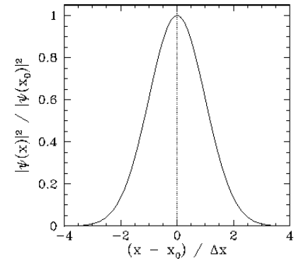
For instance, suppose that at $t=0$ the wavefunction of our particle takes the form $$\label{e2.45} \psi(x,0) \propto \exp\left[{\rm i}\,k_0\,x - \frac{(x-x_0)^{\,2}}{4\,({\mit\Delta}x)^{\,2}}\right].$$ Thus, the initial probability density of the particle is written $$\label{e2.46} |\psi(x,0)|^{\,2} \propto \exp\left[- \frac{(x-x_0)^{\,2}}{2\,({\mit\Delta}x)^{\,2}}\right].$$ This particular probability distribution is called a Gaussian distribution, and is plotted in Figure [f4]. It can be seen that a measurement of the particle’s position is most likely to yield the value $x_0$, and very unlikely to yield a value which differs from $x_0$ by more than $3\,{\mit\Delta} x$. Thus, Equation ([e2.45]) is the wavefunction of a particle that is initially localized around $x=x_0$ in some region whose width is of order ${\mit\Delta} x$. This type of wavefunction is known as a wave-packet.

Figure 7: A Gaussian probability distribution in -space.

According to Equation ([e2.42]), $$\psi(x,0) = \int_{-\infty}^{\infty} \bar{\psi}(k)\,{\rm e}^{\,{\rm i}\,k\,x}\,dk.$$ Hence, we can employ Fourier’s theorem to invert this expression to give $$\label{e2.42a} \bar{\psi}(k)\propto \int_{-\infty}^{\infty} \psi(x,0)\,{\rm e}^{-{\rm i}\,k\,x}\,dx.$$ Making use of Equation ([e2.45]), we obtain $$\bar{\psi}(k) \propto {\rm e}^{-{\rm i}\,(k-k_0)\,x_0}\int_{-\infty}^{\infty} \exp\left[ -{\rm i}\,(k-k_0)\,(x-x_0) - \frac{(x-x_0)^{\,2}}{4\,({\mit\Delta}x)^{\,2}}\right]dx.$$ Changing the variable of integration to $y=(x-x_0)/ (2\,{\mit\Delta} x)$, this reduces to $$\bar{\psi}(k) \propto {\rm e}^{-{\rm i}\,k\,x_0} \int_{-\infty}^{\infty}\exp\left(-{\rm i}\,\beta\,y - y^{\,2}\right) dy,$$ where $\beta = 2\,(k-k_0)\,{\mit\Delta}x$. The previous equation can be rearranged to give $$\bar{\psi}(k) \propto {\rm e}^{-{\rm i}\,k\,x_0 - \beta^{\,2}/4}\int_{-\infty}^{\infty} {\rm e}^{-(y-y_0)^{\,2}}\,dy,$$ where $y_0 = - {\rm i}\,\beta/2$. The integral now just reduces to a number, as can easily be seen by making the change of variable $z=y-y_0$. Hence, we obtain $$\label{e2.51} \bar{\psi}(k) \propto \exp\left[-{\rm i}\,k\,x_0 - \frac{(k-k_0)^{\,2}}{4\,({\mit\Delta}k)^{\,2}}\right],$$ where $${\mit\Delta} k = \frac{1}{2\,{\mit\Delta} x}.$$

If $|\psi(x)|^{\,2}$ is proportional to the probability density of a measurement of the particle’s position yielding the value $x$ then it stands to reason that $|\bar{\psi}(k)|^{\,2}$ is proportional to the probability density of a measurement of the particle’s wavenumber yielding the value $k$. (Recall that $p = \hbar\,k$, so a measurement of the particle’s wavenumber, $k$, is equivalent to a measurement of the particle’s momentum, $p$). According to Equation ([e2.51]), $$\label{e2.53} |\bar{\psi}(k)|^{\,2} \propto \exp\left[- \frac{(k-k_0)^{\,2}}{2\,({\mit\Delta}k)^{\,2}}\right].$$ Note that this probability distribution is a Gaussian in $k$-space. [See Equation ([e2.46]) and Figure [f4].] Hence, a measurement of $k$ is most likely to yield the value $k_0$, and very unlikely to yield a value which differs from $k_0$ by more than $3\,{\mit\Delta}k$. Incidentally, a Gaussian is the only simple mathematical function in $x$-space that has the same form as its Fourier transform in $k$-space.

We have just seen that a Gaussian probability distribution of characteristic width ${\mit\Delta} x$ in $x$-space [see Equation ([e2.46])] transforms to a Gaussian probability distribution of characteristic width ${\mit\Delta} k$ in $k$-space [see Equation ([e2.53])], where $${\mit\Delta}x\,{\mit\Delta} k = \frac{1}{2}.$$ This illustrates an important property of wave-packets. Namely, if we wish to construct a packet that is very localized in $x$-space (i.e., if ${\mit\Delta}x$ is small) then we need to combine plane-waves with a very wide range of different $k$-values (i.e., ${\mit\Delta}k$ will be large). Conversely, if we only combine plane-waves whose wavenumbers differ by a small amount (i.e., if ${\mit\Delta}k$ is small) then the resulting wave-packet will be very extended in $x$-space (i.e., ${\mit\Delta}x$ will be large).

Contributors and Attributions

• Richard Fitzpatrick (Professor of Physics, The University of Texas at Austin)

  $\newcommand {\ltapp} {\stackrel {_{\normalsize<}}{_{\normalsize \sim}}}$ $\newcommand {\gtapp} {\stackrel {_{\normalsize>}}{_{\normalsize \sim}}}$ $\newcommand {\btau}{\mbox{\boldmath$\tau$}}$ $\newcommand {\bmu}{\mbox{\boldmath$\mu$}}$ $\newcommand {\bsigma}{\mbox{\boldmath$\sigma$}}$ $\newcommand {\bOmega}{\mbox{\boldmath$\Omega$}}$ $\newcommand {\bomega}{\mbox{\boldmath$\omega$}}$ $\newcommand {\bepsilon}{\mbox{\boldmath$\epsilon$}}$