
8.3: Hydrogen Atom

( \newcommand{\kernel}{\mathrm{null}\,}\)
A hydrogen atom consists of an electron, of charge −e and mass me, and a proton, of charge +e and mass mp, moving in the Coulomb potential V(r)=−e24πϵ0|r|, where r is the position vector of the electron with respect to the proton. Now, according to the analysis in Section [stwo], this two-body problem can be converted into an equivalent one-body problem. In the latter problem, a particle of mass μ=mempme+mp moves in the central potential V(r)=−e24πϵ0r. Note, however, that because me/mp≃1/1836 the difference between me and μ is very small. Hence, in the following, we shall write neglect this difference entirely.
Writing the wavefunction in the usual form, ψ(r,θ,ϕ)=Rn,l(r)Yl,m(θ,ϕ), it follows from Section 1.2 that the radial function Rn,l(r) satisfies −ℏ22me[d2dr2+2rddr−l(l+1)r2]Rn,l−(e24πϵ0r+E)Rn,l=0. Let r=az, with
a=√ℏ22me(−E)=√E0Ea0, where E0 and a0 are defined in Equations ([e9.56]) and ([e9.57]), respectively. Here, it is assumed that E<0, because we are only interested in bound-states of the hydrogen atom. The previous differential equation transforms to [d2dz2+2zddz−l(l+1)z2+ζz−1]Rn,l=0, where
ζ=2meae24πϵ0ℏ2=2√E0E. Suppose that Rn,l(r)=Z(r/a)exp(−r/a)/(r/a). It follows that
[d2dz2−2ddz−l(l+1)z2+ζz]Z=0. We now need to solve the previous differential equation in the domain z=0 to z=∞, subject to the constraint that Rn,l(r) be square-integrable.
Let us look for a power-law solution of the form
Z(z)=∑kckzk. Substituting this solution into Equation ([e9.48]), we obtain ∑kck{k(k−1)zk−2−2kzk−1−l(l+1)zk−2+ζzk−1}=0. Equating the coefficients of zk−2 gives the recursion relation
ck[k(k−1)−l(l+1)]=ck−1[2(k−1)−ζ]. Now, the power series ([e9.49]) must terminate at small k, at some positive value of k, otherwise Z(z) behaves unphysically as z→0 [i.e., it yields an Rn,l(r) that is not square integrable as r→0]. From the previous recursion relation, this is only possible if [kmin(kmin−1)−l(l+1)]=0, where the first term in the series is ckminzkmin. There are two possibilities: kmin=−l or kmin=l+1. However, the former possibility predicts unphysical behavior of Z(z) at z=0. Thus, we conclude that kmin=l+1. Note that, because Rn,l(r)≃Z(r/a)/(r/a)≃(r/a)l at small r, there is a finite probability of finding the electron at the nucleus for an l=0 state, whereas there is zero probability of finding the electron at the nucleus for an l>0 state [i.e., |ψ|2=0 at r=0, except when l=0].
For large values of z, the ratio of successive coefficients in the power series ([e9.49]) is ckck−1=2k, according to Equation ([e9.51]). This is the same as the ratio of successive coefficients in the power series ∑k(2z)kk!, which converges to exp(2z). We conclude that Z(z)→exp(2z) as z→∞. It thus follows that Rn,l(r)∼Z(r/a)exp(−r/a)/(r/a)→exp(r/a)/(r/a) as r→∞. This does not correspond to physically acceptable behavior of the wavefunction, because ∫|ψ|2dV must be finite. The only way in which we can avoid this unphysical behavior is if the power series ([e9.49]) terminates at some maximum value of k. According to the recursion relation ([e9.51]), this is only possible if
ζ2=n, where n is an integer, and the last term in the series is cnzn. Because the first term in the series is cl+1zl+1, it follows that n must be greater than l, otherwise there are no terms in the series at all. Finally, it is clear from Equations ([e9.45]), ([e9.47]), and ([e9.54]) that
E0=−mee42(4πϵ0)2ℏ2=−e28πϵ0a0=−13.6eV, and
a0=4πϵ0ℏ2mee2=5.3×10⁻¹¹m. Here, E0 is the energy of so-called ground-state (or lowest energy state) of the hydrogen atom, and the length a0 is known as the Bohr radius. Note that |E0|∼α2mec2, where α=e2/(4πϵ0ℏc)≃1/137 is the dimensionless fine-structure constant. The fact that |E0|≪mec2 is the ultimate justification for our non-relativistic treatment of the hydrogen atom.
We conclude that the wavefunction of a hydrogen atom takes the form
ψn,l,m(r,θ,ϕ)=Rn,l(r)Yl,m(θ,ϕ). Here, the Yl,m(θ,ϕ) are the spherical harmonics (see Section [sharm]), and Rn,l(z=r/a) is the solution of [1z2ddzz2ddz−l(l+1)z2+2nz−1]Rn,l=0 which varies as zl at small z. Furthermore, the quantum numbers n, l, and m can only take values that satisfy the inequality
|m|≤l<n, where n is a positive integer, l a non-negative integer, and m an integer.
We expect the stationary states of the hydrogen atom to be orthonormal: that is, ∫ψ∗n′,l′,m′ψn,l,mdV=δnn′δll′δmm′, where dV is a volume element, and the integral is over all space. Of course, dV=r2drdΩ, where dΩ is an element of solid angle. Moreover, we already know that the spherical harmonics are orthonormal [see Equation ([spho])]: that is, ∮Y∗l′,m′Yl,mdΩ=δll′δmm′. It, thus, follows that the radial wavefunction satisfies the orthonormality constraint ∫∞0R∗n′,lRn,lr2dr=δnn′. The first few radial wavefunctions for the hydrogen atom are listed below: R1,0(r)=2a3/20exp(−ra0),R2,0(r)=2(2a0)3/2(1−r2a0)exp(−r2a0),R2,1(r)=1√3(2a0)3/2ra0exp(−r2a0),R3,0(r)=2(3a0)3/2(1−2r3a0+2r227a20)exp(−r3a0),R3,1(r)=4√29(3a0)3/2ra0(1−r6a0)exp(−r3a0),R3,2(r)=2√227√5(3a0)3/2(ra0)2exp(−r3a0). These functions are illustrated in Figures [coul1] and [coul2].
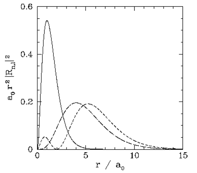
Figure 21: The a0r2|Rn,l(r)|2 plotted as a functions of r/a0. The solid, short-dashed, and long-dashed curves correspond to n,l=1,0, and 2,0, and 2,1, respectively.
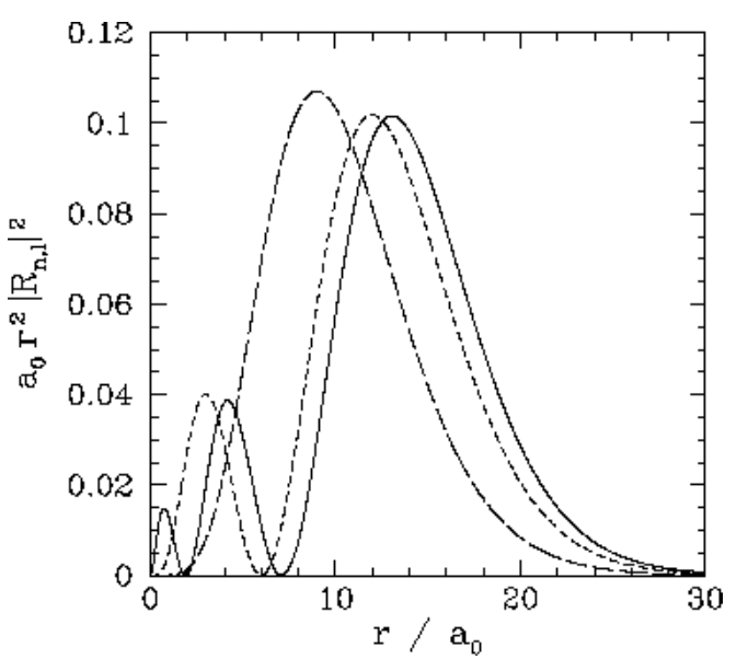
Figure 22: The a0r2|Rn,l(r)|2 plotted as a functions of r/a0.The solid, short-dashed, and long-dashed curves correspond to n,l=3,0, and 3,1, and 3,2, respectively.
Given the (properly normalized) hydrogen wavefunction ([e9.59]), plus our interpretation of |ψ|2 as a probability density, we can calculate ⟨rk⟩=∫∞0r2+k|Rn,l(r)|2dr, where the angle-brackets denote an expectation value. For instance, it can be demonstrated (after much tedious algebra) that
⟨r2⟩=a20n22[5n2+1−3l(l+1)],⟨r⟩=a02[3n2−l(l+1)],⟨1r⟩=1n2a0,⟨1r2⟩=1(l+1/2)n3a20,⟨1r3⟩=1l(l+1/2)(l+1)n3a30.
According to Equation ([e9.55]), the energy levels of the bound-states of a hydrogen atom only depend on the radial quantum number n. It turns out that this is a special property of a 1/r potential. For a general central potential, V(r), the quantized energy levels of a bound-state depend on both n and l. (See Section 1.3.)
The fact that the energy levels of a hydrogen atom only depend on n, and not on l and m, implies that the energy spectrum of a hydrogen atom is highly degenerate: that is, there are many different states which possess the same energy. According to the inequality ([e9.61]) (and the fact that n, l, and m are integers), for a given value of l, there are 2l+1 different allowed values of m (i.e., −l,−l+1,⋯,l−1,l). Likewise, for a given value of n, there are n different allowed values of l (i.e., 0,1,⋯,n−1). Now, all states possessing the same value of n have the same energy (i.e., they are degenerate). Hence, the total number of degenerate states corresponding to a given value of n is 1+3+5+⋯+2(n−1)+1=n2. Thus, the ground-state (n=1) is not degenerate, the first excited state (n=2) is four-fold degenerate, the second excited state (n=3) is nine-fold degenerate, et cetera (Actually, when we take into account the two spin states of an electron, the degeneracy of the nth energy level becomes 2n2.)
Contributors and Attributions
Richard Fitzpatrick (Professor of Physics, The University of Texas at Austin)