3.1: Quantum Interference and the AB Effect

In the past two chapters, we have already discussed some effects of the de Broglie wave interference. For example, standing waves inside a potential well, or even on the top of a potential barrier, may be considered as a result of interference of incident and reflected waves. However, there are some remarkable new effects made possible by spatial separation of such waves, and such separation requires a higher (either 2D or 3D) dimensionality. A good example of wave separation is provided by the Young-type experiment (Fig. 1) in which particles, emitted by the same source, are passed through two narrow holes (or slits) is an otherwise opaque partition.

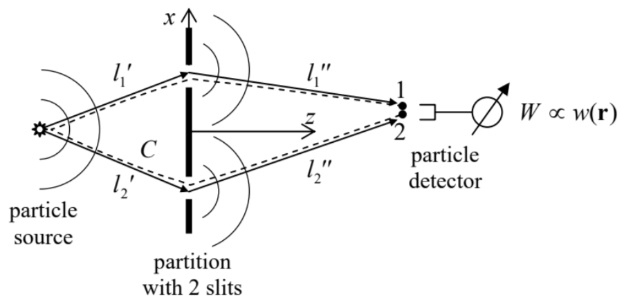Fig. 3.1. The scheme of the “two-slit” (Young-type) interference experiment.

According to Eq. (1.22), if particle interactions are negligible (which is always true if the emission rate is sufficiently low), the average rate of particle counting by the detector is proportional to the probability density \(w(\mathbf{r}, t)=\Psi(\mathbf{r}, t) \Psi *(\mathbf{r}, t)\) to find a single particle at the detector’s location \(\mathbf{r}\), where \(\Psi(\mathbf{r}, t)\) is the solution of the single-particle Schrödinger equation (1.25) for the system. Let us calculate the rate for the case when the incident particles may be represented by virtuallymonochromatic waves of energy \(E\) (e.g., very long wave packets), so that their wavefunction may be taken in the form given by Eqs. (1.57) and (1.62): \(\Psi(\mathbf{r}, t)=\psi(\mathbf{r}) \exp \{-i E t / \hbar\}\). In this case, in the freespace parts of the system, where \(U(\mathbf{r})=0, \psi(\mathbf{r})\) satisfies the stationary Schrödinger equation (1.78a): \[-\frac{\hbar^{2}}{2 m} \nabla^{2} \psi=E \psi\] With the standard definition \(k \equiv(2 m E)^{1 / 2} / \hbar\), it may be rewritten as the 3D Helmholtz equation: \[\nabla^{2} \psi+k^{2} \psi=0 .\] The opaque parts of the partition may be well described as classically forbidden regions, so if their size scale \(a\) is much larger than the wavefunction penetration depth \(\delta\) described by Eq. (2.59), we may use on their surface \(S\) the same boundary conditions as for the well’s walls of infinite height: \[\left.\psi\right|_{S}=0 .\] Eqs. (1) and (2) describe the standard boundary problem of the theory of propagation of scalar waves of any nature. For an arbitrary geometry, this problem does not have a simple analytical solution. However, for a conceptual discussion of wave interference, we may use certain natural assumptions that will allow us to find its particular, approximate solution.

First, let us discuss the wave emission, into free space, by a small-size, isotropic source located at the origin of our reference frame. Naturally, the emitted wave should be spherically symmetric: \(\psi(\mathbf{r})\) \(=\psi(r)\). Using the well-known expression for the Laplace operator in spherical coordinates, \({ }^{1}\) we may reduce Eq. (1) to the following ordinary differential equation: \[\frac{1}{r^{2}} \frac{d}{d r}\left(r^{2} \frac{d \psi}{d r}\right)+k^{2} \psi=0\] Let us introduce a new function, \(f(r) \equiv r \psi(r)\). Plugging the reciprocal relation \(\psi=f / r\) into Eq. (3), we see that it is reduced to the 1D wave equation, \[\frac{d^{2} f}{d r^{2}}+k^{2} f=0 \text {. }\] As was discussed in Sec. 2.2, for a fixed \(k\), the general solution of Eq. (4) may be represented in the form of two traveling waves: \[f=f_{+} e^{i k r}+f_{-} e^{-i k r}\] so that the full wavefunction is \[\psi(\mathbf{r})=\frac{f_{+}}{r} e^{i k r}+\frac{f_{-}}{r} e^{-i k r}, \text { i.e. } \Psi(\mathbf{r}, t)=\frac{f_{+}}{r} e^{i(k r-\omega t)}+\frac{f_{-}}{r} e^{-i(k r+\omega t)}, \quad \text { with } \omega \equiv \frac{E}{\hbar}=\frac{\hbar k^{2}}{2 m} .\] If the source is located at point \(\mathbf{r}^{\prime} \neq 0\), the obvious generalization of Eq. (6) is \[\Psi(\mathbf{r}, t)=\frac{f_{+}}{R} e^{i(k R-\omega t)}+\frac{f_{-}}{R} e^{-i(k R+\omega t)}, \quad \text { with } R \equiv|\mathbf{R}|, \quad \mathbf{R} \equiv \mathbf{r}-\mathbf{r}^{\prime} .\] The first term of this solution describes a spherically-symmetric wave propagating from the source outward, while the second one, a wave converging onto the source point \(\mathbf{r}\) ’ from large distances. Though the latter solution is possible at some very special circumstances (say, when the outgoing wave is reflected back from a spherical shell), for our current problem, only the outgoing waves are relevant, so that we may keep only the first term (proportional to \(f_{+}\)) in Eq. (7). Note that the factor \(R\) is the denominator (that was absent in the 1D geometry) has a simple physical sense: it provides the independence of the full probability current \(I=4 \pi R^{2} j(R)\), with \(j(R) \propto k \Psi \Psi^{*} \propto 1 / R^{2}\), of the distance \(R\) between the observation point and the source.

Now let us assume that the partition’s geometry is not too complicated - for example, it is either planar as shown in Fig. 1, or nearly-planar, and consider the region of the particle detector location far behind the partition (at \(z \gg 1 / k\) ), and at a relatively small angle to it: \(|x|<<z\). Then it should be physically clear that the spherical waves (7) emitted by each point inside the slit cannot be perturbed too much by the opaque parts of the partition, and their only role is the restriction of the set of such emitting points to the area of the slits. Hence, an approximate solution of the boundary problem is given by the following Huygens principle: the wave behind the partition looks as if it was the sum of contributions (7) of point sources located in the slits, with each source’s strength \(f_{+}\)proportional to the amplitude of the wave arriving at this pseudo-source from the real source - see Fig. 1. This principle finds its confirmation in the strict wave theory, which shows that with our assumptions, the solution of the boundary problem (1)-(2) may be represented as the following Kirchhoff integral: \(^{2}\) \[\psi(\mathbf{r})=c \int_{\text {slits }} \frac{\psi\left(\mathbf{r}^{\prime}\right)}{R} e^{i k R} d^{2} r^{\prime}, \quad \text { with } c=\frac{k}{2 \pi i} .\] If the source is also far from the partition, its wave’s front is almost parallel to the slit plane, and if the slits are not too broad, we can take \(\psi\left(\mathbf{r}^{\prime}\right)\) constant \(\left(\psi_{1,2}\right)\) at each slit, so that Eq. (8) is reduced to \[\psi(\mathbf{r})=a^{\prime \prime}{ }_{1} \exp \left\{i k l^{\prime \prime}{ }_{1}\right\}+a_{2}^{\prime \prime} \exp \left\{i k l_{2}^{\prime \prime}\right\}, \quad \text { with } a_{1,2}^{\prime \prime}=\frac{c A_{1,2}}{l_{1,2}^{\prime \prime}} \psi_{1,2},\] where \(A_{1,2}\) are the slit areas, and \(l\) ", \(_{1,2}\) are the distances from the slits to the detector. The wavefunctions on the slits may be calculated approximately \(^{3}\) by applying the same Eq. (7) to the region before the slits: \(\psi_{1,2} \approx\left(f_{+} / l^{\prime}{ }_{1,2}\right) \exp \left\{i k l^{\prime}{ }_{1,2}\right\}\), where \(l_{1,2}^{\prime}\) are the distances from the source to the slits - see Fig. 1. As a result, Eq. (9) may be rewritten as \[\psi(\mathbf{r})=a_{1} \exp \left\{i k l_{1}\right\}+a_{2} \exp \left\{i k l_{2}\right\}, \quad \text { with } l_{1,2} \equiv l_{1,2}^{\prime}+l_{1,2}^{\prime \prime} ; \quad a_{1,2} \equiv \frac{c f_{+} A_{1,2}}{l_{1,2}^{\prime} l_{1,2}^{\prime \prime}} .\] (As Fig. 1 shows, each of \(l_{1,2}\) is the full length of the classical path of the particle from the source, through the corresponding slit, and further to the observation point \(\mathbf{r}\).)

According to Eq. (10), the resulting rate of particle counting at point \(\mathbf{r}\) is proportional to

where \[\begin{gathered} w(\mathbf{r})=\psi(\mathbf{r}) \psi^{*}(\mathbf{r})=\left|a_{1}\right|^{2}+\left|a_{2}\right|^{2}+2\left|a_{1} a_{2}\right| \cos \varphi_{12}, \\ \varphi_{12} \equiv k\left(l_{2}-l_{1}\right) \end{gathered}\] is the difference of the total wave phase accumulations along each of two alternative paths. The last expression may be evidently generalized as \[\varphi_{12}=\oint_{C} \mathbf{k} \cdot d \mathbf{r},\] with integration along the virtually closed contour \(C\) (see the dashed line in Fig. 1), i.e. from point 1, in the positive (i.e. counterclockwise) direction all the way to point 2 . (From our discussion of the 1D WKB approximation in Sec. \(2.4\), we may expect such generalization to be valid even if \(k\) changes, sufficiently slowly, along the paths.)

Our result (11)-(12) shows that the particle counting rate oscillates as a function of the difference \(\left(l_{2}-l_{1}\right)\), which in turn changes with the detector’s position, giving the famous interference pattern, with the amplitude proportional to the product \(\left|a_{1} a_{2}\right|\), and hence vanishing if any of the slits is closed. For the wave theory, this is a well-known result, \({ }^{4}\) but for particle physics, it was (and still is :-) rather shocking. Indeed, our analysis is valid for a very low particle emission rate, so that there is no other way to interpret the pattern other than resulting from a particle’s interference with itself - or rather the interference of its de Broglie waves passing through each of two slits. \({ }^{5}\) Nowadays, such interference is reliably observed not only for electrons but also for much heavier particles: atoms and molecules, including very complex organic ones; \({ }^{6}\) moreover, atomic interferometers are used as ultra-sensitive instruments for measurements of gravity, rotation, and tilt. \({ }^{7}\)

Let us now discuss a very interesting effect of magnetic field on quantum interference. To simplify our discussion, let us consider a slightly different version of the two-slit experiment, in which each of the two alternative paths is constricted to a narrow channel using partial confinement - see Fig. 2. (In this arrangement, moving the particle detector without changing channels’ geometry, and hence local values of \(k\) may be more problematic experimentally, so let us think about its position \(\mathbf{r}\) as fixed.) In this case, because of the effect of the walls providing the path confinement, we cannot use Eqs. (10) for the amplitudes \(a_{1,2}\). However, from the discussions in Sec. \(1.6\) and Sec. 2.2, it should be clear that the first of the expressions (10) remains valid, though maybe with a value of \(k\) specific for each channel.

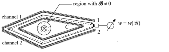Fig. 3.2. The AB effect.

In this geometry, we can apply some local magnetic field \(\mathscr{R}\), say normal to the plane of particle motion, whose lines would pierce, but not touch the contour \(C\) drawn along the particle propagation channels - see the dashed line in Fig. 2. In classical electrodynamics, \({ }^{8}\) the external magnetic field’s effect on a particle with electric charge \(q\) is described by the Lorentz force \[\mathbf{F}_{\mathscr{B}}=q \mathbf{v} \times \mathscr{B},\] where \(\mathscr{R}\) is the field value at the point of its particle’s location, so that for the experiment shown in Fig. \(2, \mathbf{F}_{\mathscr{B}}=0\), and the field would not affect the particle motion at all. In quantum mechanics, this is not so, and the field does affect the probability density \(w\), even if \(\mathscr{B}=0\) at all points where the wavefunction \(\psi(\mathbf{r})\) is not equal to zero.

In order to describe this surprising effect, let us first develop a general framework for an account of electromagnetic field effects on a quantum particle, which will also give us some by-product results important for forthcoming discussions. To do that, we need to calculate the Hamiltonian of a charged particle in electric and magnetic fields. For an electrostatic field, this is easy. Indeed, from classical electrodynamics we know that such field may be represented as a gradient of its electrostatic potential \(\phi\), \[\mathscr{E}=-\nabla \phi(\mathbf{r}),\] so that the force exerted by the field on a particle with electric charge \(q\), \[\mathbf{F}_{\varepsilon}=q \mathscr{E},\] may be described by adding the field-induced potential energy, \[U(\mathbf{r})=q \phi(\mathbf{r}),\] to other (possible) components of the full potential energy of the particle. As was already discussed in Sec. 1.4, such potential energy may be included in the particle’s Hamiltonian operator just by adding it to the kinetic energy operator - see Eq. (1.41).

However, the magnetic field’s effect is peculiar: since its Lorentz force (14) cannot do any work on a classical particle: \[\ d \mathscr{W}_{\mathscr{B}} \equiv \mathbf{F}_{\mathscr{B}} \cdot d \mathbf{r}=\mathbf{F}_{\mathscr{B}} \cdot \mathbf{v} d t=q(\mathbf{v} \times \mathscr{B}) \cdot \mathbf{v} d t=0,\] the field cannot be represented by any potential energy, so it may not be immediately clear how to account for it in the Hamiltonian. The crucial help comes from the analytical-mechanics approach to classical electrodynamics: \({ }^{9}\) in the non-relativistic limit, the Hamiltonian function of a particle in an electromagnetic field looks like that in the electric field only: \[H=\frac{m v^{2}}{2}+U=\frac{p^{2}}{2 m}+q \phi \text {; }\] however, the momentum \(\mathbf{p} \equiv m \mathbf{v}\) that participates in this expression is now the difference \[\mathbf{p}=\mathbf{P}-q \mathbf{A} \text {. }\] Here \(\mathbf{A}\) is the vector potential, defined by the well-known relations for the electric and magnetic fields: 10 \[\mathscr{E}=-\nabla \phi-\frac{\partial \mathbf{A}}{\partial t}, \quad \mathscr{B}=\nabla \times \mathbf{A},\] while \(\mathbf{P}\) is the canonical momentum, whose Cartesian components may be calculated (in classics) from the Lagrangian function \(L\) using the standard formula of analytical mechanics, \[P_{j} \equiv \frac{\partial L}{\partial v_{j}} .\] To emphasize the difference between the two momenta, \(\mathbf{p}=m \mathbf{v}\) is frequently called the kinematic momentum (or " \(m \mathbf{v}\)-momentum"). The distinction between \(\mathbf{p}\) and \(\mathbf{P}=\mathbf{p}+q \mathbf{A}\) becomes more clear if we notice that the vector potential is not gauge-invariant: according to the second of Eqs. (21), at the so-called gauge transformation \[\mathbf{A} \rightarrow \mathbf{A}+\nabla \chi,\] with an arbitrary single-valued scalar gauge function \(\chi=\chi(\mathbf{r}, t)\), the magnetic field does not change. Moreover, according to the first of Eqs. (21), if we make the simultaneous replacement \[\phi \rightarrow \phi-\frac{\partial \chi}{\partial t},\] the gauge transformation does not affect the electric field either. With that, the gauge function’s choice does not affect the classical particle’s equation of motion, and hence the velocity \(\mathbf{v}\) and momentum \(\mathbf{p}\). Hence, the kinematic momentum is gauge-invariant, while \(\mathbf{P}\) is not, because according to Eqs. (20) and (23), the introduction of \(\chi\) changes it by \(q \nabla \chi\).

Now the standard way of transfer to quantum mechanics is to treat the canonical rather than kinematic momentum as prescribed by the correspondence postulate discussed in Sec. 1.2. This means that in the wave mechanics, the operator of this variable is still given by Eq. (1.26): \({ }^{11}\) \[\hat{\mathbf{P}}=-i \hbar \nabla \text {. }\] Hence the Hamiltonian operator corresponding to the classical function (19) is \[\hat{H}=\frac{1}{2 m}(-i \hbar \nabla-q \mathbf{A})^{2}+q \phi \equiv-\frac{\hbar^{2}}{2 m}\left(\nabla-\frac{i q}{\hbar} \mathbf{A}\right)^{2}+q \phi,\] so that the stationary Schrödinger equation (1.60) of a particle moving in an electromagnetic field (but Charged
particle otherwise free) is \[-\frac{\hbar^{2}}{2 m}\left(\nabla-\frac{i q}{\hbar} \mathbf{A}\right)^{2} \psi+q \phi \psi=E \psi,\] We may now repeat all the calculations of Sec. \(1.4\) for the case \(\mathbf{A} \neq 0\), and get the following generalized expression for the probability current density:

\[\mathbf{j}=\frac{\hbar}{2 i m}\left[\psi^{*}\left(\nabla-\frac{i q}{\hbar} \mathbf{A}\right) \psi-\text { c.c }\right] \equiv \frac{1}{2 m}\left[\psi^{*} \hat{\mathbf{p}} \psi-\text { c.c }\right] \equiv \frac{\hbar}{m}|\psi|^{2}\left(\nabla \varphi-\frac{q}{\hbar} \mathbf{A}\right)\] We see that the current density is gauge-invariant (as required for any observable) only if the wavefunction’s phase \(\varphi\) changes as \[\varphi \rightarrow \varphi+\frac{q}{\hbar} \chi\] This may be a point of conceptual concern: since quantum interference is described by the spatial dependence of the phase \(\varphi\), can the observed interference pattern depend on the gauge function’s choice? (That would not make any sense, because we may change the gauge in our mind.) Fortunately, this is not true, because the spatial phase difference between two interfering paths, participating in Eq. (12), is gauge-transformed as \[\varphi_{12} \rightarrow \varphi_{12}+\frac{q}{\hbar}\left(\chi_{2}-\chi_{1}\right)\] But \(\chi\) has to be a single-valued function of coordinates, hence in the limit when the points 1 and 2 coincide, \(\chi_{1}=\chi_{2}\), so that \(\Delta \varphi\) gauge-invariant, and so is the interference pattern.

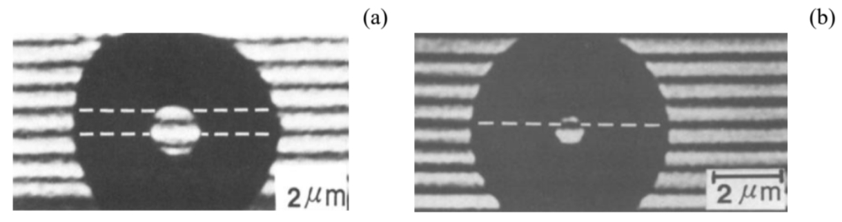
However, the difference \(\varphi\) may be affected by the magnetic field, even if it is localized outside the channels in which the particle propagates. Indeed, in this case, the field cannot affect the particle’s velocity \(\mathbf{v}\) and the probability current density \(\mathbf{j}\) : \[\left.\mathbf{j}(\mathbf{r})\right|_{\mathscr{B} \neq 0}=\left.\mathbf{j}(\mathbf{r})\right|_{\mathscr{B}=0},\] so that the last form of Eq. (28) yields \[\left.\nabla \varphi(\mathbf{r})\right|_{\mathscr{B} \neq 0}=\left.\nabla \varphi(\mathbf{r})\right|_{\mathscr{B}=0}+\frac{q}{\hbar} \mathbf{A} .\] Integrating this equation along the contour \(C\) (Fig. 2), for the phase difference between points 1 and 2 we get \[\left.\varphi_{12}\right|_{\mathscr{B} \neq 0}=\left.\varphi_{12}\right|_{\mathscr{B}=0}+\frac{q}{\hbar} \oint_{C} \mathbf{A} \cdot d \mathbf{r},\] where the integral should be taken along the same contour \(C\) as before (in Fig. 2, from point 1, counterclockwise along the dashed line to point 2). But from classical electrodynamics we know \(^{12}\) that as points 1 and 2 tend to each other, i.e. the contour \(C\) becomes closed, the last integral is just the magnetic flux \(\Phi \equiv \int \mathscr{B}_{n} d^{2} r\) through any smooth surface limited by the contour, so that Eq. (33) may be rewritten as \[\left.\varphi_{12}\right|_{\mathscr{B} \neq 0}=\left.\varphi_{12}\right|_{\mathscr{B}=0}+\frac{q}{\hbar} \Phi .\] In terms of the interference pattern, this means a shift of interference fringes, proportional to the magnetic flux (Fig. 3).

Fig. 3.3. Typical results of a two-paths interference experiment by A. Tonomura et al., Phys. Rev. Lett. 56, 792 (1986), showing the AB effect for electrons well shielded from the applied magnetic field. In this particular experimental geometry, the \(\mathrm{AB}\) effect produces a relative shift of the interference patterns inside and outside the dark ring. (a) \(\Phi=\Phi_{0}^{\prime} / 2\), (b) \(\Phi=\Phi_{0}^{\prime}\). (c) 1986 APS.

This phenomenon is usually called the "Aharonov-Bohm" (or just the \(A B\) ) effect. \({ }^{13}\) For particles with a single elementary charge, \(q=\pm e\), this result is frequently represented as \[\left.\varphi_{12}\right|_{\mathscr{B} \neq 0}=\left.\varphi_{12}\right|_{\mathscr{B}=0} \pm 2 \pi \frac{\Phi}{\Phi_{0}{ }^{\prime}},\] where the fundamental constant \(\Phi_{0}{ }^{\prime} \equiv 2 \pi \hbar / e \approx 4.14 \times 10^{-15} \mathrm{~Wb}\) has the meaning of the magnetic flux necessary to change \(\varphi_{12}\) by \(2 \pi\), i.e. to shift the interference pattern (11) by one period, and is called the normal magnetic flux quantum - "normal" because of the reasons we will soon discuss.

The \(A B\) effect may be "almost explained" classically, in terms of Faraday’s electromagnetic induction. Indeed, a change \(\Delta \Phi\) of magnetic flux in time induces a vortex-like electric field \(\Delta \mathscr{E}\) around it. That field is not restricted to the magnetic field’s location, i.e. may reach the particle’s trajectories. The field’s magnitude (or rather of its integral along the contour \(C\) ) may be readily calculated by integration of the first of Eqs. (21): \[\Delta V \equiv \oint_{C} \Delta \mathscr{E} \cdot d \mathbf{r}=-\frac{d \Phi}{d t}\] I hope that in this expression the reader readily recognizes the integral ("undergraduate") form of Faraday’s induction law. \({ }^{14}\) To calculate the effect of this electric field of the particles, let us assume that the variable separation described by Eq. (1.57) may be applied to the end points 1 and 2 of particle’s alternative trajectories as two independent systems, \({ }^{15}\) and that the magnetic flux’ change by a certain amount \(\Delta \Phi\) does not change the spatial factors \(\psi_{1,2}\), with the phases \(\varphi_{1,2}\) included into the timedependent factors \(a_{1,2}\). Then we may repeat the arguments that were used in Sec. \(1.6\) at the discussion of the Josephson effect, and since the change (35) leads to the change of the potential energy difference \(\Delta U\) \(=q \Delta V\) between the two points, we may rewrite Eq. (1.72) as \[\frac{d \varphi_{12}}{d t}=-\frac{\Delta U}{\hbar}=-\frac{q}{\hbar} \Delta V=\frac{q}{\hbar} \frac{d \Phi}{d t} .\] Integrating this relation over the time of the magnetic field’s change, we get \[\Delta \varphi_{12}=\frac{q}{\hbar} \Delta \Phi,\]

• superficially, the same result as given by Eq. (34).

However, this interpretation of the \(\mathrm{AB}\) effect is limited. Indeed, it requires the particle to be in the system (on the way from the source to the detector) during the flux change, i.e. when the induced electric field \(\mathscr{E}\) may affect its dynamics. On the contrary, Eq. (34) predicts that the interference pattern would shift even if the field change has been made when there was no particle in the system, and hence the field \(\mathscr{E}\) could not be felt by it. Experiment confirms the latter conclusion. Hence, there is something in the space where a particle propagates (i.e., outside of the magnetic field region), that transfers the information about even the static magnetic field to the particle. The standard interpretation of this surprising fact is as follows: the vector potential \(\mathbf{A}\) is not just a convenient mathematical tool, but a physical reality (just as its scalar counterpart \(\phi\) ), despite the large freedom of choice we have in prescribing specific spatial and temporal dependences of these potentials without affecting any observable - see Eqs. (23)-(24).To conclude this section, let me briefly discuss the very interesting form taken by the \(\mathrm{AB}\) effect in superconductivity. To be applied to this case, our results require two changes. The first one is simple: since superconductivity may be interpreted as the Bose-Einstein condensate of Cooper pairs with electric charge \(q=-2 e, \Phi_{0}\) ’ has to be replaced by the so-called superconducting flux quantum \(^{16}\) \[\Phi_{0} \equiv \frac{\pi \hbar}{e} \approx 2.07 \times 10^{-15} \mathrm{~Wb}=2.07 \times 10^{-7} \mathrm{Gs} \cdot \mathrm{cm}^{2} .\] Second, since the pairs are Bose particles and are all condensed in the same (ground) quantum state, described by the same wavefunction, the total electric current density, proportional to the probability current density \(j\), may be extremely large - in practical superconducting materials, up to \(\sim 10^{12} \mathrm{~A} / \mathrm{m}^{2}\). In these conditions, one cannot neglect the contribution of that current into the magnetic field and hence into its flux \(\Phi\), which (according to the Lenz rule of the Faraday induction law) tries to compensate for changes in external flux. To see possible results of this contribution, let us consider a closed superconducting loop (Fig. 4). Due to the Meissner effect (which is just another version of the flux self-compensation), the current and magnetic field penetrate into a superconductor by only a small distance (called the London penetration depth) \(\delta_{\mathrm{L}} \sim 10^{-7} \mathrm{~m} .{ }^{17}\) If the loop is made of a superconducting "wire" that is considerably thicker than \(\delta_{\mathrm{L}}\), we may draw a contour deep inside the wire, at that the current density is negligible. According to the last form of Eq. (28), everywhere at the contour, \[\nabla \varphi-\frac{q}{\hbar} \mathbf{A}=0 .\] Integrating this equation along the contour as before (in Fig. 4, from some point 1, all the way around the ring to the virtually coinciding point 2), we need to have the phase difference \(\varphi_{12}\) equal to \(2 \pi n\), because the wavefunction \(\psi \propto \exp \{i \varphi\}\) in the initial and final points 1 and 2 should be "essentially" the same, i.e. produce the same observables. As a result, we get \[\Phi \equiv \oint_{C} \mathbf{A} \cdot d \mathbf{r}=\frac{\hbar}{q} 2 \pi n \equiv n \Phi_{0} .\] This is the famous flux quantization effect, \({ }^{18}\) which justifies the term "magnetic flux quantum" for the constant \(\Phi_{0}\) given by Eq. (38).

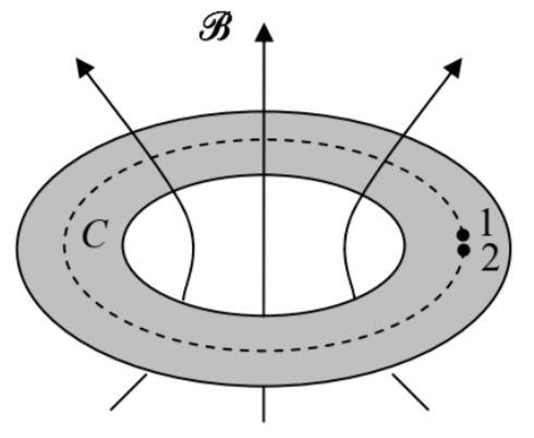Fig. 3.4. The magnetic flux quantization in a superconducting loop (schematically).

Unfortunately, in this course I have no space/time to discuss the very interesting effects of "partial flux quantization" that arise when a superconductor loop is closed with a Josephson junction, forming the so-called Superconductor QUantum Interference Device - "SQUID". Such devices are used, in particular, for supersensitive magnetometry and ultrafast, low-power computing. \({ }^{19}\)

---

\({ }^{1}\) See, e.g., MA Eq. (10.9) with \(\partial / \partial \theta=\partial / \partial \varphi=0\).

\({ }^{2}\) For the proof and a detailed discussion of Eq. (8), see, e.g., EM Sec. \(8.5\).

\({ }^{3}\) A possible (and reasonable) concern about the application of Eq. (7) to the field in the slits is that it ignores the effect of opaque parts of the partition. However, as we know from Chapter 2, the main role of the classically forbidden region is reflecting the incident wave toward its source (i.e. to the left in Fig. 1). As a result, the contribution of this reflection to the field inside the slits is insignificant if \(A_{1,2}>>\lambda^{2}\), and even in the opposite case provides just some rescaling of the amplitudes \(a_{1,2}\), which is not important for our conceptual discussion.

\({ }^{4}\) See, e.g., a detailed discussion in EM Sec. 8.4.

\({ }^{5}\) Here I have to mention the fascinating experiments (first performed in 1987 by C. Hong et al. with photons, and recently, in 2015 , by R. Lopes et al., with non-relativistic particles - helium atoms) on the interference of de Broglie waves of independent but identical particles, in the same internal quantum state and virtually the same values of \(E\) and \(k\). These experiments raise the important issue of particle indistinguishability, which will be discussed in Sec. 8.1.

\({ }^{6}\) See, e.g., the recent demonstration of the quantum interference of oligo-porphyrin molecules, consisting of 2,000 atoms, with a total mass above \(25,000 m_{\mathrm{p}}-\) Y. Fein et al., Nature Physics 15, 1242 (2019).

\({ }^{7}\) See, e.g., the review paper by A. Cronin, J. Schmiedmayer, and D. Pritchard, Rev. Mod. Phys. 81, 1051 (2009).

\({ }^{8}\) See, e.g., EM Sec. 5.1. Note that Eq. (14), as well as all other formulas of this course, are in the SI units.

\({ }^{9}\) See, e.g., EM Sec. 9.7, in particular Eq. (9.196).

\({ }^{10}\) See, e.g., EM Sec. 6.1, in particular Eqs. (6.7).

\({ }^{11}\) The validity of this choice is clear from the fact that if the kinetic momentum was described by this differential operator, the Hamiltonian operator corresponding to the classical Hamiltonian function (19), and the corresponding Schrödinger equation would not describe the magnetic field effects at all.

\({ }^{12}\) See, e.g., EM Sec. 5.3.

\({ }^{13}\) I prefer the latter, less personable name, because the effect had been actually predicted by Werner Ehrenberg and Raymond Siday in 1949, before it was rediscovered (also theoretically) by Y Aharonov and D. Bohm in 1959. To be fair to Aharonov and Bohm, it was their work that triggered a wave of interest in the phenomenon, resulting in its first experimental observation by Robert G. Chambers in 1960 and several other groups soon after that. Later, the experiments were improved using ferromagnetic cores and/or superconducting shielding to provide a better separation between the electrons and the applied field \(-\) as in the work whose result is shown in Fig. \(3 .\)

\({ }^{14}\) See, e.g., EM Sec. 6.1.

\({ }^{15}\) This assumption may seem a little bit of a stretch, but the resulting relation (37) may be indeed proven for a rather realistic model, though that would take more time/space than I can afford.

\({ }^{16}\) One more bad, though common term: a metallic wire may (super)conduct, but a quantum hardly can!

\({ }^{17}\) For more detail, see EM Sec. 6.4.

\({ }^{18}\) It was predicted in 1949 by Fritz London and experimentally discovered (independently and virtually simultaneously) in 1961 by two experimental groups: B. Deaver and W. Fairbank, and R. Doll and M. Näbauer.

\({ }^{19}\) A brief review of these effects, and recommendations for further reading may be found in EM Sec. 6.5.