3.2: Landau Levels and the Quantum Hall Effect

In the last section, we have used the Schrödinger equation (27) for an analysis of static magnetic field effects in "almost-1D", circular geometries shown in Figs. 1, 2, and 4. However, this equation describes very interesting effects in fully-higher-dimensions as well, especially in the \(2 \mathrm{D}\) case. Let us consider a quantum particle free to move in the \([x, y]\) plane only (say, due to its strong confinement in the perpendicular direction \(z\) - see the discussion in Sec. 1.8). Taking the confinement energy for the reference, we may reduce Eq. (27) to a similar equation, but with the Laplace operator acting only in the directions \(x\) and \(y\) : \[-\frac{\hbar^{2}}{2 m}\left(\mathbf{n}_{x} \frac{\partial}{\partial x}+\mathbf{n}_{y} \frac{\partial}{\partial y}-i \frac{q}{\hbar} \mathbf{A}\right)^{2} \psi=E \psi .\] Let us find its solutions for the simplest case when the applied static magnetic field is uniform and perpendicular to the motion plane: \[\mathscr{B}=\mathscr{B} \mathbf{n}_{z} .\] According to the second of Eqs. (21), this relation imposes the following restriction on the choice of the vector potential: \[\frac{\partial A_{y}}{\partial x}-\frac{\partial A_{x}}{\partial y}=\mathscr{R},\] but the gauge transformations still give us a lot of freedom in its choice. The "natural" axiallysymmetric form, \(\mathbf{A}=\mathbf{n}_{\varphi} \rho \mathscr{B} / 2\), where \(\rho=\left(x^{2}+y^{2}\right)^{1 / 2}\) is the distance from some \(z\)-axis, leads to cumbersome math. In 1930, L. Landau realized that the energy spectrum of Eq. (41) may be obtained by making a much simpler, though very counter-intuitive choice: \[A_{x}=0, \quad A_{y}=\mathscr{B}\left(x-x_{0}\right),\] (with arbitrary \(x_{0}\) ), which evidently satisfies Eq. (43), though ignores the physical symmetry of the \(x\) and \(y\) directions for the field (42).

Now, expanding the eigenfunction into the Fourier integral in the \(y\)-direction: \[\psi(x, y)=\int X_{k}(x) \exp \left\{i k\left(y-y_{0}\right)\right\} d k,\] we see that for each component of this integral, Eq. (41) yields a specific equation \[-\frac{\hbar^{2}}{2 m}\left\{\mathbf{n}_{x} \frac{d}{d x}+i \mathbf{n}_{y}\left[k-\frac{q}{\hbar} \mathscr{B}\left(x-x_{0}\right)\right]\right\}^{2} X_{k}=E X_{k} .\] Since the two vectors inside the curly brackets are mutually perpendicular, its square has no cross-terms, so that Eq. (46) reduces to \[-\frac{\hbar^{2}}{2 m} \frac{d^{2}}{d x^{2}} X_{k}+\frac{q^{2}}{2 m} \mathscr{B}^{2}\left(x-x_{0}{ }^{\prime}\right)^{2} X_{k}=E X_{k}, \quad \text { where } x_{0}{ }^{\prime} \equiv x_{0}+\frac{\hbar k}{q \mathscr{B}} .\] But this 1D Schrödinger equation is identical to Eq. (2.261) for a 1D harmonic oscillator, \({ }^{20}\) with the center at point \(x_{0}{ }^{\prime}\), and frequency \(\omega_{0}\) equal to \[\omega_{\mathrm{c}}=\frac{|q \mathscr{B}|}{m} .\] In the last expression, it is easy to recognize the cyclotron frequency of the classical particle’s rotation in the magnetic field. (It may be readily obtained using the \(2^{\text {nd }}\) Newton law for a circular orbit of radius \(r\), \[m \frac{v^{2}}{r}=F_{\text {क }} \equiv q v \mathscr{R},\] and noting that the resulting ratio \(v / r=|q \mathscr{R}| / m\) is just the radius-independent angular velocity \(\omega_{\mathrm{c}}\) of the particle’s rotation.) Hence, the energy spectrum for each Fourier component of the expansion (45) is the same:

\[E_{n}=\hbar \omega_{\mathrm{c}}\left(n+\frac{1}{2}\right)\] independent of either \(x_{0}\), or \(y_{0}\), or \(k\).

This is a good example of a highly degenerate system: for each eigenvalue \(E_{n}\), there are many similar eigenfunctions that differ only by the positions \(\left\{x_{0}, y_{0}\right\}\) of their centers, and the rate \(k\) of their phase change along the \(y\)-axis. They may be used to assemble a large variety of linear combinations, including 2D wave packets whose centers move along classical circular orbits. Note, however, that the radius of such rotation cannot be smaller than the so-called Landau radius, \[r_{\mathrm{L}} \equiv\left(\frac{\hbar}{m \omega_{\mathrm{c}}}\right)^{1 / 2} \equiv\left(\frac{\hbar}{|q \mathscr{B}|}\right)^{1 / 2},\] which characterizes the minimum size of the wave packet, and follows from Eq. (2.276) after the replacement \(\omega_{0} \rightarrow \omega_{\mathrm{c}}\). This radius is remarkably independent of the particle mass, and may be interpreted in the following way: the scale \(\mathscr{R} A_{\min }\) of the applied magnetic field’s flux through the effective area \(A_{\min }=2 \pi r_{\mathrm{L}}^{2}\) of the smallest wave packet is just one normal flux quantum \(\Phi_{0}{ }^{\prime} \equiv 2 \pi \hbar /|q|\).

A detailed analysis of such wave packets (for which we would not have time in this course), in particular proves the virtually evident fact: the applied magnetic field does not change the average density \(d N_{2} / d E\) of different \(2 \mathrm{D}\) states on the energy scale, following from Eq. (1.99), but just "assembles" them on the Landau levels (see Fig. 5a), so that the number of different orbital states on each Landau level (per unit area) is \[n_{\mathrm{L}} \equiv \frac{N_{2}}{A}=\left.\left.\frac{1}{A} \frac{d N_{2}}{d E}\right|_{\mathscr{B}=0} \Delta E \equiv \frac{1}{A} \frac{d N_{2}}{d^{2} k}\right|_{\mathscr{B}=0} \frac{d^{2} k}{d k} \frac{1}{d E / d k} \Delta E=\frac{1}{A} \frac{A}{(2 \pi)^{2}} 2 \pi k \frac{1}{\hbar^{2} k / m} \hbar \omega_{\mathrm{c}} \equiv \frac{|q \mathscr{B}|}{2 \pi \hbar} .\] This expression may again be interpreted in terms of magnetic flux quanta: \(n_{\mathrm{L}} \Phi_{0}{ }^{\prime}=\mathscr{B}\), i.e. there is one particular state on each Landau level per each normal flux quantum.

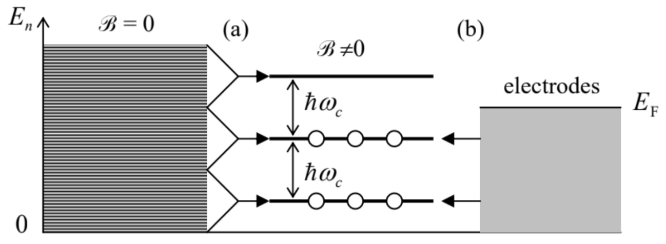Fig. 3.5. (a) The “assembly” of 2D states on Landau levels, and (b) filling the levels with electrons at the quantum Hall effect.

The most famous application of the Landau levels picture is the explanation of the quantum Hall effect \({ }^{21}\). It is usually observed in the "Hall bar" geometry sketched in Fig. 6 , where electric current \(I\) is passed through a rectangular conducting sample placed into magnetic field \(\mathscr{R}\) perpendicular to the sample’s plane. The classical analysis of the effect is based on the notion of the Lorentz force (14). As the magnetic field is turned on, this force starts to deviate the effective charge carriers (electrons or holes) from their straight motion between the electrodes, bending them toward the insulated sides of the bar (in Fig. 6, parallel to the \(x\)-axis). Here the carriers accumulate, generating a gradually increasing electric field \(\mathscr{E}\) until its force (16) exactly balances the Lorentz force (14): \[q \mathscr{E}_{y}=q v_{x} \mathscr{B},\] where \(v_{x}\) is the drift velocity of the carriers along the bar (Fig. 6), providing the sustained balance condition \(\mathscr{E}_{y} / v_{x}=\mathscr{B}\) at each point of the sample.

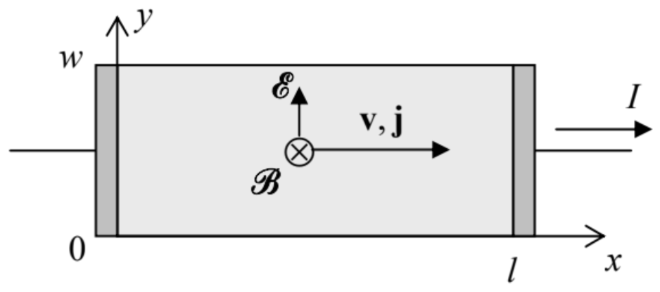Fig. 3.6. The Hall bar geometry. Darker rectangles show external (3D) electrodes.

With \(n_{2}\) carriers per unit area, in a sample of width \(w\), this condition yields the following classical expression for the so-called Hall resistance \(R_{\mathrm{H}}\), remarkably independent of \(w\) and \(l\) : \[R_{\mathrm{H}} \equiv \frac{V_{y}}{I_{x}}=\frac{\mathscr{E}_{y} w}{q n_{2} v_{x} w}=\frac{\mathscr{R}}{q n_{2}} .\] This formula is broadly used in practice for the measurement of the \(2 \mathrm{D}\) density \(n_{2}\) of the charge carriers, and of the carrier type \(-\) electrons with \(q=-e<0\), or holes with the effective charge \(q=+e>0\).

However, in experiments with high-quality (low-defect) 2D well structures, at sub-kelvin temperatures 22 and high magnetic fields, the linear growth of \(R_{\mathrm{H}}\) with \(\mathscr{B}\), described by Eq. (54), is interrupted by virtually horizontal plateaus (Fig. 7). Most remarkably, the experimental values of \(R_{\mathrm{H}}\) on these plateaus are reproduced with extremely high accuracy (up to \(\sim 10^{-9}\) ) from experiment to experiment and, even more remarkably, from sample to sample. \({ }^{23}\) They are described by the following formula: \[R_{\mathrm{H}}=\frac{1}{i} R_{\mathrm{K}}, \quad \text { where } R_{\mathrm{K}} \equiv \frac{2 \pi \hbar}{e^{2}},\] so that \[R_{\mathrm{K}} \approx 25.812807459304 \ldots \mathrm{k} \Omega,\] and \(i\) is (only until the end of this section, following tradition!) the plateau number, i.e. a real integer.

Fig. 3.7. A typical record of the integer quantum Hall effect. The lower trace (with sharp peaks) shows the diagonal component, \(V_{x} / I_{x}\), of the resistance tensor. (Adapted from https://www.nobelprize.org/nobel_prizes/physics/laureates/1998/press.html).

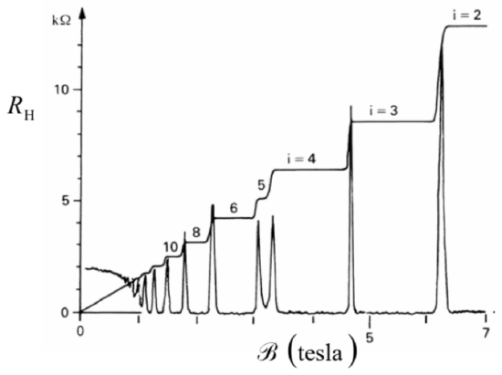
This effect may be explained using the Landau level picture. The 2D sample is typically in a weak contact with 3D electrodes whose conductivity electrons, at low temperatures, fill all states with energies below a certain Fermi energy \(E_{\mathrm{F}}\) - see Fig. \(5 \mathrm{~b}\). According to Eqs. (48) and (50), as \(\mathscr{R}\) is increased, the spacing \(\hbar \omega_{\mathrm{c}}\) between the Landau levels increases proportionately, so that fewer and fewer of these levels are below \(E_{\mathrm{F}}\) (and hence all their states are filled in equilibrium), and within certain ranges of field variations, the number \(i\) of the filled levels is constant. (In Fig. 5b, \(i=2\).) So, plugging \(n_{2}\) \(=i n_{\mathrm{L}}\) and \(q=-e\) into Eq. (54), and using Eq. (52) for \(n_{\mathrm{L}}\), we get \[R_{\mathrm{H}}=\frac{1}{i} \frac{\mathscr{B}}{q n_{\mathrm{L}}}=\frac{1}{i} \frac{2 \pi \hbar}{e^{2}},\] i.e. exactly the experimental result (55).

This admittedly oversimplified explanation of the quantum Hall effect does not take into account at least two important factors:

(i) the nonuniformity of the background potential \(U(x, y)\) in realistic Hall bar samples, and the role of the quasi-1D edge channels this nonuniformity produces \(;{ }^{24}\) and

(ii) the Coulomb interaction of the electrons, in high-quality samples leading to the formation of \(R_{\mathrm{H}}\) plateaus with not only integer but also fractional values of \(i\left(1 / 3,2 / 5,3 / 7\right.\), etc.). \({ }^{25}\)

Unfortunately, a thorough discussion of these very interesting features is well beyond the framework of this course. \({ }^{26 \cdot 27}\)

---

\({ }^{20}\) This result may become a bit less puzzling if we recall that at the classical circular cyclotron motion of a particle, each of its Cartesian coordinates, including \(x\), performs sinusoidal oscillations with frequency (48), just as a 1D harmonic oscillator with this frequency.

\({ }^{21}\) It was first observed in 1980 by a group led by Klaus von Klitzing, while the classical version (54) of the effect was first observed by Edwin Hall a century earlier - in \(1879 .\)

\({ }^{22}\) In some systems, such as the graphene (virtually perfect 2D sheets of carbon atoms - see Sec. 4 below), the effect may be more stable to thermal fluctuations, due to their topological properties, so that it may be observed even at room temperature \(-\) see, e.g., K. Novoselov et al., Science 315,1379 (2007). Also note that in some thin ferromagnetic layers, the quantum Hall effects may be observed in the absence of an external magnetic field - see, e.g., M. Götz et al., Appl. Phys. Lett. 112, 072102 (2018) and references therein.

\({ }^{23}\) Due to this high accuracy (which is a rare exception in solid-state physics!), since 2018 the von Klitzing constant \(R_{\mathrm{K}}\) is used in metrology for the "legal" ohm’s definition, with its value (56) considered fixed - see Appendix CA: Selected Physical Constants.

\({ }^{24}\) Such quasi-1D regions, with the width of the order of \(r_{\mathrm{L}}\), form along the lines where the Landau levels cross the Fermi surface, and are actually responsible for all the electron transfer at the quantum Hall effect (giving the pioneering example of what is nowadays called the topological insulators). The particle motion along these channels is effectively one-dimensional; because of this, it cannot be affected by modest unintentional nonuniformities of the potential \(U(x, y)\). This fact is responsible for the extraordinary accuracy of Eq. (55).

\({ }^{25}\) This fractional quantum Hall effect was discovered in 1982 by D. Tsui, H. Stormer, and A. Gossard. In contrast, the effect described by Eq. (55) with an integer \(i\) (Fig. 7) is now called the integer quantum Hall effect. \({ }^{26}\) For a comprehensive discussion of these effects, I can recommend, e.g., either the monograph by D. Yoshioka, The Quantum Hall Effect, Springer, 1998, or the review by D. Yennie, Rev. Mod. Phys. 59, 781 (1987). (See also the later publications cited above.)

\({ }^{27}\) Note also that the quantum Hall effect is sometimes discussed in terms of the so-called Berry phase, one of the geometric phases - the notion apparently pioneered by S. Pancharatnam in 1956. However, in the "usual" quantum Hall effect the Berry phase equals zero, and I believe that this concept should be saved for the discussion of more topologically involved systems. Unfortunately, I will have no time/space for a discussion of such systems in this course, and have to refer the interested reader to special literature - see, e.g., either the key papers collected by A. Shapere and F. Wilczek, Geometric Phases in Physics, World Scientific, 1992, or the monograph by A. Bohm et al., The Geometric Phase in Quantum Systems, Springer, \(2003 .\)