3.8: Spherically-symmetric Scatterers

The machinery of the Legendre polynomials and the spherical Bessel functions, discussed in Sec. 6 , may also be used for analysis of particle scattering by spherically-symmetric potentials (155) beyond the Born approximation (Sec. 3), provided that such a potential \(U(r)\) is also localized, i.e. reduces sufficiently fast at \(r \rightarrow \infty\). (The quantification of this condition is left for the reader’s exercise.)

Indeed, directing the \(z\)-axis along the propagation of the incident plane de Broglie wave \(\psi_{\mathrm{i}}\), and taking its origin in the center of the scatterer, we may expect the scattered wave \(\psi_{\text {s }}\) to be axially symmetric, so that its expansion in the series over the spherical harmonics includes only the terms with \(m=0\). Hence, the solution (64) of the stationary Schrödinger equation (63) in this case may be represented as \({ }^{91}\) \[\psi=\psi_{\mathrm{i}}+\psi_{\mathrm{s}}=a_{\mathrm{i}}\left[e^{i k z}+\sum_{l=0}^{\infty} R_{l}(r) P_{l}(\cos \theta)\right],\]

where \(k \equiv(2 m E)^{1 / 2} / \hbar\) is defined by the energy \(E\) of the incident particle, while the radial functions \(R_{l}(r)\) have to satisfy Eq. (181), and be finite at \(r \rightarrow 0\). At large distances \(r \gg R\), where \(R\) is the effective radius of the scatterer, the potential \(U(r)\) is negligible, and Eq. (181) is reduced to Eq. (183). In contrast to its analysis in Sec. 6, we should look for its solution using a linear superposition of the spherical Bessel functions of both kinds: \[R_{l}(r)=A_{l} j_{l}(k r)+B_{l} y_{l}(k r), \quad \text { at } r \gg>R,\] because Eq. (183) is now invalid at \(r \rightarrow 0\), and our former argument for dropping the functions \(y_{l}(k r)\) is no more valid. In Eq. (214), \(A_{l}\) and \(B_{l}\) are some complex coefficients, determined by the scattering potential \(U(r)\), i.e. by the solution of Eq. (181) at \(r \sim R\).

As the explicit expressions (186) show, the spherical Bessel functions \(j_{l}(\xi)\) and \(y_{l}(\xi)\) represent standing de Broglie waves, with equal real amplitudes, so that their simple linear combinations (called the spherical Hankel functions of the first and second kind), \[h_{l}^{(1)}(\xi) \equiv j_{l}(\xi)+i y_{l}(\xi), \quad \text { and } h_{l}^{(2)}(\xi) \equiv j_{l}(\xi)-i y_{l}(\xi),\] represent traveling spherical waves propagating, respectively, from the origin (i.e. from the center of the scatterer), and toward the origin. In particular, at \(\xi>>1, l\), i.e. at large distances \(r \gg 1 / k, l / k, 92\) \[h_{l}^{(1)}(k r) \rightarrow \frac{(-i)^{l+1}}{k r} e^{i k r} \quad h_{l}^{(2)}(k r) \rightarrow \frac{i^{l+1}}{k r} e^{-i k r} .\] But using the same physical argument as at the beginning of Sec. 1, we may argue that in the case of a localized scatterer, there should be no latter waves at \(r \gg R\); hence, we have to require the amplitude of the term proportional to \(h_{l}^{(2)}\) to be zero. With the relations reciprocal to Eqs. (215), \[j_{l}(\xi)=\frac{1}{2}\left[h_{l}^{(1)}(\xi)+h_{l}^{(2)}(\xi)\right], \quad y_{l}(\xi)=\frac{1}{2 i}\left[h_{l}^{(1)}(\xi)-h_{l}^{(2)}(\xi)\right]\] which enable us to rewrite Eq. (214) as \[\begin{aligned} R_{l}(r) &=\frac{A_{l}}{2}\left[h_{l}^{(1)}(\xi)+h_{l}^{(2)}(\xi)\right]+\frac{B_{l}}{2 i}\left[h_{l}^{(1)}(\xi)-h_{l}^{(2)}(\xi)\right] \\ & \equiv\left(\frac{A_{l}-i B_{l}}{2}\right) h_{l}^{(1)}(\xi)+\left(\frac{A_{l}+i B_{l}}{2}\right) h_{l}^{(2)}(\xi), \end{aligned}\] this means that the combination \(\left(A_{l}+i B_{l}\right)\) has to be equal zero, so that \(B_{l}=i A_{l}\). Hence we have just one unknown coefficient (say, \(A_{l}\) ) for each \(l,{ }^{93}\) and may rewrite Eq. (218) in an even simpler form: \[R_{l}(r)=A_{l}\left[j_{l}(k r)+i y_{l}(k r)\right] \equiv A_{l} h_{l}^{(1)}(k r), \quad \text { at } r \gg>R,\] and use Eqs. (213) and (216) to write the following expression for the scattered wave at large distances: \[\psi_{\mathrm{s}} \approx \frac{a_{\mathrm{i}}}{k r} e^{i k r} \sum_{l=0}^{\infty}(-i)^{l+1} A_{l} P_{l}(\cos \theta), \quad \text { at } r>>R, \frac{1}{k}, \frac{l}{k} .\] Comparing this expression with the general Eq. (81), we see that for a spherically-symmetric, localized scatterer, \[f=\frac{1}{k} \sum_{l=0}^{\infty}(-i)^{l+1} A_{l} P_{l}(\cos \theta),\] so that the differential cross-section (84) is \[\frac{d \sigma}{d \Omega}=\frac{1}{k^{2}}\left|\sum_{l=0}^{\infty}(-i)^{l+1} A_{l} P_{l}(\cos \theta)\right|^{2} \equiv \frac{1}{k^{2}} \sum_{l, l^{\prime}=0}^{\infty} i^{l^{\prime}-l} A_{l} A_{l^{\prime}}^{*} P_{l}(\cos \theta) P_{l}(\cos \theta) .\] The last expression is more convenient for the calculation of the total cross-section \((59)\) : \[\sigma=\oint_{4 \pi} \frac{d \sigma}{d \Omega} d \Omega=2 \pi \int_{-1}^{+1} \frac{d \sigma}{d \Omega} d(\cos \theta)=\frac{2 \pi}{k^{2}} \sum_{l, l=0}^{\infty} i^{l^{\prime}-l} A_{l} A_{l^{\prime}}^{*} \int_{-1}^{+1} P_{l}(\xi) P_{l^{\prime}}(\xi) d \xi,\] where \(\xi \equiv \cos \theta\), because this result may be much simplified by using Eq. (167): \({ }^{94}\) \[\ \text{Spherically-symmetric scatterer:}\sigma\quad\quad\quad\quad\sigma=\sum_{l=0}^{\infty} \sigma_{l}, \quad \text { with } \sigma_{l}=\frac{4 \pi}{k^{2}} \frac{\left|A_{l}\right|^{2}}{2 l+1}.\] Hence the solution of the scattering problem is reduced to the calculation of the partial wave amplitudes \(A_{l}\) defined by Eq. (219) - and for the total cross-section, merely of their magnitudes. This task is much facilitated by using the following Rayleigh formula for the expansion of the incident plane wave’s exponent into a series over the Legendre polynomials, \({ }^{95}\) \[\ e^{i k z} \equiv e^{i k r \cos \theta}=\sum_{l=0}^{\infty} i^{l}(2 l+1) j_{l}(k r) P_{l}(\cos \theta).\] As the simplest example, let us calculate scattering by a completely opaque and "hard" (meaning sharp-boundary) sphere, which may be described by the following potential: \[U(r)= \begin{cases}+\infty, & \text { for } r<R, \\ 0, & \text { for } R<r .\end{cases}\] In this case, the total wavefunction has to vanish at \(r \leq R\), and hence for the external problem \((r \geq R)\) the sphere enforces the boundary condition \(\psi \equiv \psi_{0}+\psi_{\mathrm{s}}=0\) for all values of \(\theta\), at \(r=R\). With Eqs. (213), (220) and (225), this condition becomes \[a_{\mathrm{i}} \sum_{l=0}^{\infty}\left[R_{l}(R)+i^{l}(2 l+1) j_{l}(k R)\right] P_{l}(\cos \theta)=0 .\] Due to the orthogonality of the Legendre polynomials, this condition may be satisfied for all angles \(\theta\) only if all the coefficients before all \(P_{l}(\cos \theta)\) vanish, i.e. if \[R_{l}(R)=-i^{l}(2 l+1) j_{l}(k R) .\] On the other hand, for \(r>R, U(r)=0\), so that Eq. (183) is valid, and its outward-wave solution (219) has to be valid even at \(r \rightarrow R\), giving \[R_{l}(R)=A_{l}\left[j_{l}(k R)+i y_{l}(k R)\right] .\] Requiring the two last expressions to give the same result, we get \[A_{l}=-i^{l}(2 l+1) \frac{j_{l}(k R)}{j_{l}(k R)+i y_{l}(k R)},\] so that Eqs. (222) and (224) yield: \[\frac{d \sigma}{d \Omega}=\frac{1}{k^{2}}\left|\sum_{l=0}^{\infty}(2 l+1) \frac{j_{l}(k R)}{j_{l}(k R)+i y_{l}(k R)} P_{l}(\cos \theta)\right|^{2}, \quad \sigma_{l}=\frac{4 \pi(2 l+1)}{k^{2}} \frac{j_{l}^{2}(k R)}{j_{l}^{2}(k R)+y_{l}^{2}(k R)}\] As Fig. 25a shows, the first of these results describes an angular structure of the scattered de Broglie wave, which is qualitatively similar to that given by the Born approximation - cf. Eq. (98) and Fig. 10.

Fig. 3.25. Particle scattering by an opaque, hard sphere: (a) the differential cross-section normalized to the geometric cross-section \(\sigma_{\mathrm{g}} \equiv \pi R^{2}\) of the sphere, as a function of the scattering angle \(\theta\), and (b) the (similarly normalized) total cross-section and its lowest spherical components, as functions of the dimensionless product \(k R \propto E^{1 / 2}\).

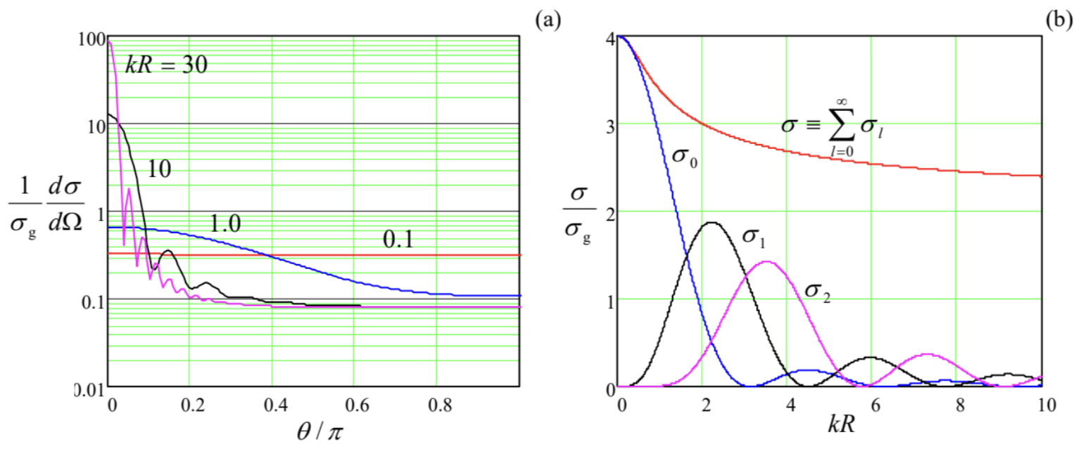
Namely, at low particle’s energies \((k R<<1)\), the scattering is essentially isotropic, while in the opposite, high-energy limit \(k R>>1\), it is mostly confined to small angles \(\theta \sim \pi / k R<<1\), and exhibits numerous local destructive-interference minima at angles \(\theta_{n} \sim \pi n / k R\). However, in our current (exact!) theory, these minima are always finite, because the theory describes effective bending of the de Broglie waves along the back side of the sphere, which smears the interference pattern. The same bending is also responsible for a rather counter-intuitive fact, described by the second of Eqs. (231) and clearly visible in Fig. 25b: even at \(k R \rightarrow \infty\), the total cross-section \(\sigma\) of scattering tends to \(2 \sigma_{\mathrm{g}} \equiv 2 \pi R^{2}\), rather than to \(\sigma_{\mathrm{g}}\) as in the purely-classical scattering theory. (The fact that at \(k R<<\) 1 , the cross-section is also larger than \(\sigma_{\mathrm{g}}\), approaching \(4 \sigma_{\mathrm{g}}\) at \(k R \rightarrow 0\), is less surprising, because in this limit the de Broglie wavelength \(\lambda=2 \pi / k\) is much longer than the sphere’s radius \(R\), so that the wave’s propagation is affected by the whole sphere.)

The above analysis may be readily generalized to the case a step-like (sharp but finite) potential (97) - the problem left for the reader’s exercise. On the other hand, for a finite and smooth scattering potential \(U(r)\), plugging Eq. (225) into Eq. (213) and the result into Eq. (66), requiring the coefficients before each angular function \(P_{l}(\cos \theta)\) to be balanced, and canceling the common coefficient \(a_{0}\), we get the following inhomogeneous generalization of Eq. (181) for the radial functions defined by Eq. (213): \[[E-U(r)] R_{1}+\frac{\hbar^{2}}{2 m r^{2}}\left[\frac{d}{d r}\left(r^{2} \frac{d}{d r}\right)-l(l+1)\right] R_{l}(r)=U(r) i^{l}(2 l+1) j_{l}(k r) .\] This differential equation has to be solved in the whole scatterer volume (i.e. for all \(r \sim R\) ) with the boundary conditions for the functions \(R_{(r)}\) to be finite at \(r \rightarrow 0\), and to tend to the asymptotic form (219) at \(r>>R\). The last requirement enables the evaluation of the coefficients \(A_{l}\) that are needed for spelling out Eqs. (222) and (224). Unfortunately, due to the lack of time, I have to refer the reader interested in such cases to special literature. \({ }^{96}\)

---

\({ }^{91}\) The particular terms in this sum are frequently called partial waves.

\({ }^{92}\) For arbitrary \(l\), this result may be confirmed using Eqs. (185) and the asymptotic formulas for the "usual" Bessel functions - see, e.g., EM Eqs. (2.135) and (2.152), valid for an arbitrary (not necessarily integer) index \(n\).

\({ }_{93}\) Moreover, using the conservation of the orbital momentum, to be discussed in Sec. 5.6, it is possible to show that this complex coefficient may be further reduced to just one real parameter, usually recast as the partial phase shift \(\delta_{l}\) between the \(l^{\text {th }}\) spherical harmonics of the incident and scattered waves. However, I will not use this notion, because practical calculations are more physically transparent (and not more complex) without it.

\({ }^{94}\) Physically, this reduction of the double sum to a single one means that due to the orthogonality of the spherical functions, the total scattering probability flows due to each partial wave just add up.

\({ }^{95}\) It may be proved using the Rodrigues formula (165) and integration by parts - the task left for the reader’s exercise.

\({ }^{96}\) See, e.g., J. Taylor, Scattering Theory, Dover, \(2006 .\)