3.7: Atoms

Now we are ready to discuss atoms, starting from the simplest, exactly solvable Bohr atom problem, i.e. that of a single particle’s motion in the so-called attractive Coulomb potential 77 \[U(r)=-\frac{C}{r}, \text { with } C>0 .\] The natural scales of \(E\) and \(r\) in this problem are commonly defined by the requirement of equality of the kinetic and potential energy magnitude scales (dropping all numerical coefficients): \[E_{0} \equiv \frac{\hbar^{2}}{m r_{0}^{2}} \equiv \frac{C}{r_{0}},\] similar to its particular case (1.13b). Solving this system of two equations, we get \({ }^{78}\) \[E_{0} \equiv \frac{\hbar^{2}}{m r_{0}^{2}} \equiv m\left(\frac{C}{\hbar}\right)^{2}, \quad \text { and } r_{0} \equiv \frac{\hbar^{2}}{m C} .\] In the normalized units \(\varepsilon \equiv E / E_{0}\) and \(\xi \equiv r / r_{0}\), equation (181) for our current case (190), looks relatively simple, \[\frac{d^{2} R}{d \xi^{2}}+\frac{2}{\xi} \frac{d R}{d \xi}-l(l+1) R+2\left(\varepsilon+\frac{1}{\xi}\right) R=0,\] but unfortunately, its eigenfunctions may be called elementary only in the most generous meaning of the word. With the adequate normalization, \[\int_{0}^{\infty} R_{n, l} R_{n^{\prime}, l} r^{2} d r=\delta_{n n^{\prime}},\] these (mutually orthogonal) functions may be represented as \[R_{n, l}(r)=-\left\{\left(\frac{2}{n r_{0}}\right)^{3} \frac{(n-l-1) !}{2 n[(n+l) !]^{3}}\right\}^{1 / 2} \exp \left\{-\frac{r}{n r_{0}}\right\}\left(\frac{2 r}{n r_{0}}\right)^{l} L_{n-l-1}^{2 l+1}\left(\frac{2 r}{n r_{0}}\right)\] Here \(L_{p}^{q}(\xi)\) are the so-called associated Laguerre polynomials, which may be calculated as \[L_{p}^{q}(\xi)=(-1)^{q} \frac{d^{q}}{d \xi^{q}} L_{p+q}(\xi)\] from the simple Laguerre polynomials \(L_{p}(\xi) \equiv L_{p}^{0}(\xi) \cdot{ }^{79}\) In turn, the easiest way to obtain \(L_{p}(\xi)\) is to use the following Rodrigues formula: \({ }^{80}\) \[\text { (3.197) }\] \[L_{p}(\xi)=e^{\xi} \frac{d^{p}}{d \xi^{p}}\left(\xi^{p} e^{-\xi}\right) .\] Note that in contrast with the associated Legendre functions \(P_{l}^{m}\), participating in the spherical harmonics, all \(L_{p}^{q}\) are just polynomials, and those with small indices \(p\) and \(q\) are indeed quite simple: \[\begin{array}{lll} L_{0}^{0}(\xi)=1, & L_{1}^{0}(\xi)=-\xi+1, & L_{2}^{0}(\xi)=\xi^{2}-4 \xi+2, \\ L_{0}^{1}(\xi)=1, & L_{1}^{1}(\xi)=-2 \xi+4, & L_{2}^{1}(\xi)=3 \xi^{2}-18 \xi+18, \\ L_{0}^{2}(\xi)=2, & L_{1}^{2}(\xi)=-6 \xi+18, & L_{2}^{2}(\xi)=12 \xi^{2}-96 \xi+144, \ldots \end{array}\] Returning to Eq. (195), we see that the natural quantization of the radial equation (193) has brought us a new integer quantum number \(n\). To understand its range, we should notice that according to Eq. (197), the highest power of terms in the polynomial \(L_{p+q}\) is \((p+q)\), and hence, according to Eq. (196), that of \(L_{p}^{q}\) is \(p\), so that the highest power in the polynomial participating in Eq. (195) is \((n-l-\) 1). Since the power cannot be negative to avoid the unphysical divergence of wavefunctions at \(r \rightarrow 0\), the radial quantum number \(n\) has to obey the restriction \(n \geq l+1\). Since \(l\), as we already know, may take values \(l=0,1,2, \ldots\), we may conclude \(n\) may only take the following values:

\[n=1,2,3, \ldots\] What makes this relation very important is the following, most surprising result: the eigenenergies corresponding to the wavefunctions (179), which are indexed with three quantum numbers: \[\psi_{n, l, m}=R_{n, l}(r) Y_{l}^{m}(\theta, \varphi),\] depend only on one of them, \(n\) : \[\varepsilon=\varepsilon_{n}=-\frac{1}{2 n^{2}}, \quad \text { i.e. } E_{n}=-\frac{E_{0}}{2 n^{2}}=-\frac{1}{2 n^{2}} m\left(\frac{C}{\hbar}\right)^{2} .\] i.e. agree with Bohr’s formula (1.12). Because of this reason, \(n\) is usually called the principal quantum number, and the above relation between it and the "more subordinate" orbital quantum number \(l\) is rewritten as \[l \leq n-1 .\] Together with the inequality (162), this gives us the following, very important hierarchy of the three quantum numbers involved in the Bohr atom problem: \[1 \leq n \leq \infty \quad \Rightarrow \quad 0 \leq l \leq n-1 \quad \Rightarrow \quad-l \leq m \leq+l\] Taking into account the \((2 l+1)\)-degeneracy related to the magnetic number \(m\), and using the well-known formula for the arithmetic progression, \({ }^{81}\) we see that the \(n^{\text {th }}\) energy level (201) has the following orbital degeneracy: \[g=\sum_{l=0}^{n-1}(2 l+1) \equiv 2 \sum_{l=0}^{n-1} l+\sum_{l=0}^{n-1} 1=2 \frac{n(n-1)}{2}+n \equiv n^{2} .\] Due to its importance for atoms, let us spell out the hierarchy (203) of a few lowest-energy states, using the traditional state notation, in which the value of \(n\) is followed by the letter that denotes the value of \(l\) : \[\begin{array}{llcc} n=1: & l=0 & \text { (one } 1 s \text { state) } & m=0 . \\ n=2: & l=0 & \text { (one } 2 s \text { state) } & m=0, \\ & l=1 & \text { (three } 2 p \text { states) } & m=0, \pm 1 . \\ n=3: & l=0 & \text { (one } 3 s \text { state) } & m=0, \\ & l=1 & \text { (three } 3 p \text { states) } & m=0, \pm 1, \\ l=2 & \text { (five } 3 d \text { states) } & m=0, \pm 1, \pm 2 . \end{array}\] Figure 22 shows plots of the radial functions (195) of the listed states. The most important of them is of course the ground \((1 s)\) state with \(n=1\) and hence \(E=-E_{0} / 2\). According to Eqs. (195) and (198), its radial function is just a simple decaying exponent \[R_{1,0}(r)=\frac{2}{r_{0}^{3 / 2}} e^{-r / r_{0}}\] while its angular distribution is uniform - see Eq. (174). The gap between the ground energy and the energy \(E=-E_{0} / 8\) of the lowest excited states (with \(n=2\) ) in a hydrogen atom (in which \(E_{0}=E_{\mathrm{H}} \approx 27.2\) \(\mathrm{eV}\) ) is as large as \(\sim 10 \mathrm{eV}\), so that their thermal excitation requires temperatures as high as \(\sim 10^{5} \mathrm{~K}\), and the overwhelming part of all hydrogen atoms in the visible Universe are in their ground state. Since the atomic hydrogen makes up about \(75 \%\) of the "normal" matter,\({ }^{82}\) we are very fortunate that such simple formulas as Eqs. (174) and (208) describe the atomic states prevalent in Mother Nature!

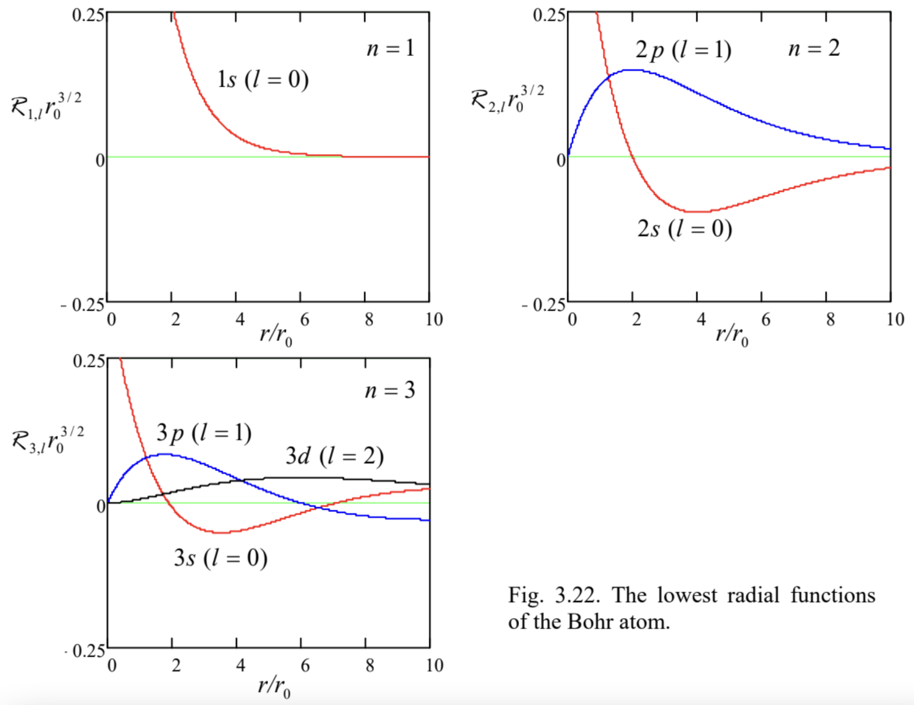Fig. 3.22. The lowest radial functions of the Bohr atom.

According to Eqs. (195) and (198), the radial functions of the lowest excited states, \(2 s\) (with \(n=\) 2 and \(l=0\) ), and \(2 p\) (with \(n=2\) and \(l=1\) ) are also not too complicated: \[R_{2,0}(r)=\frac{1}{\left(2 r_{0}\right)^{3 / 2}}\left(2-\frac{r}{r_{0}}\right) e^{-r / 2 r_{0}}, \quad R_{2,1}(r)=\frac{1}{\left(2 r_{0}\right)^{3 / 2}} \frac{r}{3^{1 / 2} r_{0}} e^{-r / 2 r_{0}},\] with the former of these states \((2 s)\) having a uniform angular distribution, and the three latter \((2 p)\) states, with different \(m=0, \pm 1\), having simple angular distributions, which differ only by their spatial orientation - see Eq. (175) and the second row of Fig. 20. The most important trend here, clearly visible from the comparison of the two top panels of Fig. 22 as well, is a larger radius of the decay exponent in the radial functions ( \(2 r_{0}\) for \(n=2\) instead of \(r_{0}\) for \(n=1\) ), and hence a larger radial extension of the states. This trend is confirmed by the following general formula: \({ }^{83}\) \[\langle r\rangle_{n, l}=\frac{r_{0}}{2}\left[3 n^{2}-l(l+1)\right] .\] The second important trend is that at a fixed \(n\), the orbital quantum number \(l\) determines how fast does the wavefunction change with \(r\) near the origin, and how much it oscillates in the radial direction at larger values of \(r\). For example, the \(2 s\) eigenfunction \(\mathcal{R}_{2,0}(r)\) is different from zero at \(r=0\), and "makes one wiggle" (has one root) in the radial direction, while the eigenfunctions \(2 p\) equal zero at \(r=0\) but do not cross the horizontal axis after that. Instead, those wavefunctions oscillate as the functions of an angle \(-\) see the second row of Fig. 20 . The same trend is clearly visible for \(n=3\) (see the bottom panel of Fig. 22), and continues for the higher values of \(n\).

The states with \(l=l_{\max } \equiv n-1\) may be viewed as crude analogs of the circular motion of a particle in a plane whose orientation defines the quantum number \(m\). On the other hand, the best classical image of the \(s\)-state \((l=0)\) is a purely radial, spherically-symmetric motion of the particle to and from the attracting center. (The latter image is especially imperfect because the motion needs to happen simultaneously in all radial directions.) The classical language becomes reasonable only for the highly degenerate Rydberg states, with \(n \gg 1\), whose linear superpositions may be used to compose wave packets closely following the classical (circular or elliptic) trajectories of the particle \(-\) just as was discussed in Sec. \(2.2\) for the free 1D motion.

Besides Eq. (210), mathematics gives us several other simple relations for the radial functions \(R_{n, l}\) (and, since the spherical harmonics are normalized to 1 , for the eigenfunctions as the whole), including those that we will use later in the course 84 \[\left\langle\frac{1}{r}\right\rangle_{n, l}=\frac{1}{n^{2} r_{0}}, \quad\left\langle\frac{1}{r^{2}}\right\rangle_{n, l}=\frac{1}{n^{3}(l+1 / 2) r_{0}^{2}}, \quad\left\langle\frac{1}{r^{3}}\right\rangle_{n, l}=\frac{1}{n^{3} l(l+1 / 2)(l+1) r_{0}^{3}} .\] In particular, the first of these formulas means that for any eigenfunction \(\psi_{n, l, m}\), with all its complicated radial and angular dependencies, there is a simple relation between the potential and full energies: \[\langle U\rangle_{n, l}=-C\left\langle\frac{1}{r}\right\rangle_{n, l}=-\frac{C}{n^{2} r_{0}}=-\frac{E_{0}}{n^{2}}=2 E_{n},\] so that the average kinetic energy of the particle, \(\langle T\rangle_{n, l}=E_{n}-\langle U\rangle_{n, l}\), is equal to \(E_{n}-2 E_{n}=\left|E_{n}\right|>0\).

As in the several previous cases we have met, simple results (201), (210)-(212) are in sharp contrast with the rather complicated expressions for the corresponding eigenfunctions. Historically this contrast gave an additional motivation for the development of more general approaches to quantum mechanics, that would replace, or at least complement our brute-force (wave-mechanics) analysis. A discussion of such an approach will be the main topic of the next chapter.

Rather strikingly, the above classification of the quantum numbers, with minor steals from the later chapters of this course, allows a semi-quantitative explanation of the whole system of chemical elements. The "only" two additions we need are the following facts:

(i) due to their unavoidable interaction with relatively low-temperature environments, atoms tend to relax into their lowest-energy state, and

(ii) due to the Pauli principle (valid for electrons as the Fermi particles), each orbital eigenstate discussed above may be occupied by two electrons with opposite spins.

Of course, atomic electrons do interact, so that their quantitative description requires quantum mechanics of multiparticle systems, which is rather complex. (Its main concepts will be discussed in Chapter 8.) However, the lion’s share of this interaction is reduced to simple electrostatic screening, i.e. a partial compensation of the electric charge of the atomic nucleus, as felt by a particular electron, by other electrons of the atom. This screening changes quantitative results (such as the energy scale \(E_{0}\) ) dramatically; however, the quantum number hierarchy, and hence their classification, is not affected.

The hierarchy of atoms is most often represented as the famous periodic table of chemical elements, \({ }^{85}\) whose simple version is shown in Fig. 23 . (The table in Fig. 24 presents a sequential list of the elements and their electron configurations, following the convention already used in Eqs. (205)(207), with the additional upper index showing the number of electrons with the indicated values of quantum numbers \(n\) and \(l\).) The number in each table’s cell, and in the first column of the list, is the socalled atomic number \(Z\), which physically is the number of protons in the particular atomic nucleus, and hence the number of electrons in an electrically-neutral atom.

Fig. 3. 23. The periodic table of elements, showing their atomic numbers and chemical symbols, as well as their color-coded basic physical/chemical properties at the so-called ambient (meaning usual laboratory) conditions.

Fig. 3.24. Atomic electron configurations. The upper index shows the number of electrons in the states with the indicated quantum numbers \(n\) (the first digit) and \(l\) (letter-coded as was discussed above). The simplest atom, with \(Z=1\), is hydrogen (chemical symbol H) - the only atom for that the theory discussed above is quantitatively correct. \({ }^{86}\) According to Eq. (191), the \(1 s\) ground state of its only electron corresponds to the quantum number values \(n=1, l=0\), and \(m=0\) - see Eq. (205). In most versions of the periodic table, the cell of \(\mathrm{H}\) is placed in the top left corner.

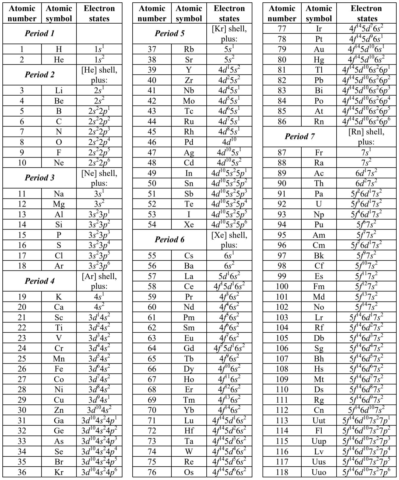
In the next atom, helium (symbol He, \(Z=2\) ), the same orbital quantum state \((1 s)\) is filled with two electrons. As will be discussed in detail in Chapter 8, electrons of the same atom are actually indistinguishable, so that their quantum states are not independent and may be entangled. These factors are important for several properties of helium atoms (and heavier elements as well); however, a bit counter-intuitively, for the atom classification purposes, they are not crucial, and we may pretend that two electrons of a helium atom just have "opposite spins". Due to the twice higher electric charge of the nucleus of the helium atom, i.e. the twice higher value of the constant \(C\) in Eq. (190), resulting in a 4fold increase of the constant \(E_{0}\) given by Eq. (192), the binding energy of each electron is crudely 4 times higher than that of the hydrogen atom - though the electron interaction decreases it by about \(25 \%\) - see Sec. 8.2. This is why taking one electron away (i.e. the positive ionization of a helium atom) requires relatively high energy, \(\sim 23.4 \mathrm{eV}\), which is not available in the usual chemical reactions. On the other hand, a neutral helium atom cannot bind one more electron (i.e. form a negative ion) either. As a result, the helium, and all other elements with fully completed electron shells (the term meaning the sets of states with eigenenergies well separated from higher energy levels) is a chemically inert noble gas, thus starting the whole right-most column of the periodic table, allocated for such elements.

The situation changes rather dramatically as we move to the next element, lithium (Li), with \(Z=\) 3 electrons. Two of them are still accommodated by the inner shell with \(n=1\) (listed in Fig. 24 as the helium shell \([\mathrm{He}])\), but the third one has to reside in the next shell with \(n=2, l=0\), and \(m=0\), i.e. in the \(2 s\) state. According to Eq. (201), the binding energy of this electron is much lower, especially if we take into account that according to Eqs. (210)-(211), the \(1 s\) electrons of the [He] shell are much closer to the nucleus and almost completely compensate two-thirds of its electric charge \(+3 e\). As a result, the \(2 s\)-state electron is approximately, but reasonably well described by Eq. (201) with \(Z=1\) and \(n=2\), giving binding energy close to just \(3.4 \mathrm{eV}\) (experimentally, \(2.39 \mathrm{eV}\) ), so that a lithium atom can give out that electron rather easily - to either an atom/ion of another element to form a chemical compound, or to the common conduction band of the solid-state lithium; as a result, at the ambient conditions, it is a typical alkali metal. The similarity of chemical properties of lithium and hydrogen, with the chemical valence of one, \({ }^{87}\) places \(\mathrm{Li}\) as the starting element of the second period (row), with the first period limited to only \(\mathrm{H}\) and \(\mathrm{He}\) - see Fig. 23 .

In the next element, beryllium (symbol Be, \(Z=4\) ), the \(2 s\) state \((n=2, l=0, m=0)\) houses one more electron, with the "opposite spin". Due to the higher electric charge of the nucleus, \(Q=+4 e\), with only half of it compensated by \(1 s\) electrons of the [He] shell, the binding energy of the \(2 s\) electrons is somewhat higher than that in lithium, so that the ionization energy increases to \(\sim 9.32 \mathrm{eV}\). As a result, beryllium is also chemically active with the valence of two, but not as active as lithium, and is also is metallic in its solid-state phase, but with a lower electric conductivity than lithium.

Moving in this way along the second row of the periodic table (from \(Z=3\) to \(Z=10\) ), we see a gradual filling of the rest of the total \(2 n^{2}=2 \times 2^{2}=8\) different electron states of the \(n=2\) shell (see Eq. (204), with the additional spin degeneracy factor of 2), including two \(2 s\) states with \(m=0\), and six \(2 p\) states with \(m=0, \pm 1,{ }^{88}\) with a gradually growing ionization potential (up to \(\sim 21.6 \mathrm{eV}\) in Ne with \(Z=\) 10), i.e. a growing reluctance to conduct electricity or form positive ions. However, the last elements of the row, such as oxygen \((\mathrm{O}\), with \(Z=8)\) and especially fluorine \((\mathrm{F}\), with \(Z=9)\) can readily pick up extra electrons to fill up their \(2 p\) states, i.e. form negative ions. As a result, these elements are chemically active, with a double valence for oxygen and a single valence for fluorine. However, the final element of this row, neon, has its \(n=2\) shell completely full, and cannot form a stable negative ion. This is why it is a noble gas, like helium. Traditionally, in the periodic table, such elements are placed right under helium (Fig. 23), to emphasize the similarity of their chemical properties. But this necessitates making an at least 6-cell gap in the \(1^{\text {st }}\) row. (Actually, the gap is often made larger, to accommodate the next rows keep reading.)

Period 3, i.e. the \(3^{\text {rd }}\) row of the table, starts exactly like period 2, with sodium (Na, with \(Z=11\) ), also a chemically active alkali metal whose atom features 10 electrons filling the shells with \(n=1\) and \(n\) \(=2\) (in Fig. 24, collectively called the neon shell [Ne]), plus one electron in the \(3 s\) state \((n=3, l=0, m=\) 0 ), which may be again reasonably well described by the hydrogen atom theory - see, e.g., the red curve on the last panel of Fig. 22. Continuing along this row, we could naively expect that, according to Eq. (204), and with the account of double spin degeneracy, this period of the table should have \(2 n^{2}=2 \times 3^{2}=\) 18 elements, with a gradual, sequential filling of two \(3 s\) states, then six \(3 p\) states, and then ten \(3 d\) states. However, here we run into a big surprise: after argon (Ar, with \(Z=18\) ), a relatively inert element with the ionization energy of \(\sim 15.7 \mathrm{eV}\) due to the fully filled \(3 s\) and \(3 p\) shells, the next element, potassium (K, with \(Z=19\) ) is an alkali metal again!

The reason for that is the difference of the actual electron energies from those of the hydrogen atom, which is due mostly to inter-electron interactions, and gradually accumulates with the growth of Z. It may be semi-quantitatively understood from the results of \(\mathrm{Sec}\). 6. In hydrogen-like atoms/ions, the electron state energies do not depend on the quantum number \(l\) (as well as \(m\) ) - see Eq. (201). However, the orbital quantum number does affect the wavefunction of an electron. As Fig. 22 shows, the larger \(l\) the less the probability for an electron to be close to the nucleus, where its positive charge is less compensated by other electrons. As a result of this effect (and also the relativistic corrections to be discussed in Sec. 6.3), the electron’s energy grows with \(l\). Actually, this effect is visible already in period 2 of the table: it manifests itself in the filling order - the \(p\) states after the \(s\) states. However, for potassium (K, with \(Z=19\) ) and calcium (Ca, with \(Z=20\) ), the energies of the \(3 d\) states become so high that the energies of the two \(4 s\) states are lower, and the latter states are filled first. As described by Eq. (210), and also by the first of Eqs. (211), the effect of the principal number \(n\) on the distance from the nucleus is much stronger than that of \(l\), so that the \(4 s\) wavefunctions of \(\mathrm{K}\) and \(\mathrm{Ca}\) are relatively far from the nucleus, and determine the chemical valence (equal to 1 and 2, correspondingly) of these elements. The next atoms, from \(\operatorname{Sc}(Z=21)\) to \(\mathrm{Zn}(Z=30)\), with the gradually filled "internal" \(3 d\) states, are the so-called transition metals whose (comparable) ionization energies and chemical properties are determined by the \(4 s\) electrons.

This fact is the origin of the difference between various forms of the "periodic" table. In its most popular option, shown in Fig. 23, \(\mathrm{K}\) is used to start the next period 4, and then a new period is started each time and only when the first electron with the next principal quantum number \((n)\) appears. \({ }^{89}\) This topology of the table provides a very clear match of the chemical properties of the first element of each period (an alkali metal), as well as its last element (a noble gas). It also automatically means making gaps in all previous rows. Usually, this gap is made between the atoms with completely filled \(s\) states and with those with the first electron in a \(p\) state, because here the properties of the elements make a somewhat larger step. (For example, the step from Be to B makes the material an insulator, but the step from \(\mathrm{Mg}\) to \(\mathrm{Al}\) makes a smaller difference.) As a result, the elements of the same column have only approximately similar chemical valences and physical properties.

In order to accommodate the lower, longer rows, such representation is inconvenient, because the whole table would be too broad. This is why the so-called rare earth elements, including lanthanides (with \(Z\) from 57 to 70 , of the \(6^{\text {th }}\) row, with a gradual filling of the \(4 f\) and \(5 d\) states) and actinides ( \(Z\) from 89 to 103 , of the \(7^{\text {th }}\) row, with a gradual filling of the \(5 f\) and \(6 d\) states), are usually represented as outlet rows \(-\) see Fig. 23. This is quite acceptable for basic chemistry, because the chemical properties of the elements within each such group are rather close.

To summarize my very short review of this extremely important topic, \({ }^{90}\) the "periodic table of elements" is not periodic in the strict sense of the word. Nevertheless, it has had an enormous historic significance for chemistry, as well as atomic and solid-state physics, and is still very convenient for many purposes. For our course, the most important aspect of its discussion is the surprising possibility to describe, at least for classification purposes, such a complex multi-electron system as an atom as a set of quasi-independent electrons in certain quantum states indexed with the same quantum numbers \(n, l\), and \(m\) as those of the hydrogen atom. This fact enables the use of various perturbation theories, which give a more quantitative description of atomic properties. Some of these techniques will be reviewed in Chapters 6 and 8.

---

\({ }^{77}\) Historically, the solution of this problem in 1928, that reproduced the main result (1.12)-(1.13) of the "old" quantum theory developed by N. Bohr in 1912, without its phenomenological assumptions, was the decisive step toward the general acceptance of Schrödinger’s wave mechanics.

\({ }^{78}\) For the most important case of the hydrogen atom, with \(C=e^{2} / 4 \pi \varepsilon_{0}\), these scales are reduced, respectively, to the Bohr radius \(r_{\mathrm{B}}(1.10)\) and the Hartree energy \(E_{\mathrm{H}}(1.13 \mathrm{a})\). Note also that according to Eq. (192), for the socalled hydrogen-like atom (actually, a positive ion) with \(C=Z\left(e^{2} / 4 \pi \varepsilon_{0}\right)\), these two key parameters are rescaled as \(r_{0}=r_{\mathrm{B}} / Z\) and \(E_{0}=\mathrm{Z}^{2} E_{\mathrm{H}}\).

\({ }^{79}\) In Eqs. (196)-(197), \(p\) and \(q\) are non-negative integers, with no relation whatsoever to the particle’s momentum or electric charge. Sorry for this notation, but it is absolutely common, and can hardly result in any confusion.

\({ }^{80}\) Named after the same B. O. Rodrigues, and belonging to the same class as his other famous result, Eq. (165) for the Legendre polynomials.

\({ }^{81}\) See, e.g., MA Eq. (2.5a).

\({ }^{82}\) Excluding the so-far hypothetical dark matter and dark energy.

\({ }^{83}\) Note that even at the largest value of \(l\), equal to \((n-1)\), the second term \(l(l+1)\) in Eq. \((210)\) is equal to \(\left(n^{2}-n\right)\), and hence cannot over-compensate the first term \(3 n^{2}\).

\({ }^{84}\) The first of these relations may be readily proved using the Heller-Feynman theorem (see Chapter 1); this proof will be offered for the reader’s exercise after a more general form of this theorem has been proved in Chapter 6.

\({ }^{85}\) Also called the Mendeleev table, after Dmitri Ivanovich Mendeleev who put forward the concept of the quasiperiodicity of chemical element properties as functions of \(Z\) phenomenologically in 1869. (The explanation of this periodicity had to wait for 60 more years until the advent of quantum mechanics in the late 1920 s.)

\({ }^{86}\) Besides very small fine-structure and hyperfine-splitting corrections - to be discussed, respectively, in Chapters 6 and \(8 .\)

\({ }^{87}\) The chemical valence (or "valency") is a not very precise term describing the number of atom’s electrons involved in chemical reactions. For the same atom, especially with a large number of electrons in its outer, unfilled shell, this number may depend on the chemical compound formed. (For example, the valence of iron is two in the ferrous oxide, \(\mathrm{FeO}\), and three in the ferric oxide, \(\mathrm{Fe}_{2} \mathrm{O}_{3}\).)

\({ }^{88}\) The specific order of filling of the states within each shell follows the so-called Hund rules - see Sec. 8.3.

\({ }^{89}\) Another popular option is to return to the first column as soon an atom has one electron in the \(s\) state (like it is in \(\mathrm{Cu}, \mathrm{Ag}\), and \(\mathrm{Au}\), in addition to the alkali metals).

\({ }_{90}\) For a bit more detailed (but still succinct) discussion of the valence and other chemical aspects of atomic structure, I can recommend Chapter 5 of the very clear text by L. Pauling, General Chemistry, Dover, \(1988 .\)