
4.4: Change of Basis, and Matrix Diagonalization
- Page ID
- 57602

\( \newcommand{\vecs}[1]{\overset { \scriptstyle \rightharpoonup} {\mathbf{#1}} } \)
\( \newcommand{\vecd}[1]{\overset{-\!-\!\rightharpoonup}{\vphantom{a}\smash {#1}}} \)
\( \newcommand{\id}{\mathrm{id}}\) \( \newcommand{\Span}{\mathrm{span}}\)
( \newcommand{\kernel}{\mathrm{null}\,}\) \( \newcommand{\range}{\mathrm{range}\,}\)
\( \newcommand{\RealPart}{\mathrm{Re}}\) \( \newcommand{\ImaginaryPart}{\mathrm{Im}}\)
\( \newcommand{\Argument}{\mathrm{Arg}}\) \( \newcommand{\norm}[1]{\| #1 \|}\)
\( \newcommand{\inner}[2]{\langle #1, #2 \rangle}\)
\( \newcommand{\Span}{\mathrm{span}}\)
\( \newcommand{\id}{\mathrm{id}}\)
\( \newcommand{\Span}{\mathrm{span}}\)
\( \newcommand{\kernel}{\mathrm{null}\,}\)
\( \newcommand{\range}{\mathrm{range}\,}\)
\( \newcommand{\RealPart}{\mathrm{Re}}\)
\( \newcommand{\ImaginaryPart}{\mathrm{Im}}\)
\( \newcommand{\Argument}{\mathrm{Arg}}\)
\( \newcommand{\norm}[1]{\| #1 \|}\)
\( \newcommand{\inner}[2]{\langle #1, #2 \rangle}\)
\( \newcommand{\Span}{\mathrm{span}}\) \( \newcommand{\AA}{\unicode[.8,0]{x212B}}\)
\( \newcommand{\vectorA}[1]{\vec{#1}} % arrow\)
\( \newcommand{\vectorAt}[1]{\vec{\text{#1}}} % arrow\)
\( \newcommand{\vectorB}[1]{\overset { \scriptstyle \rightharpoonup} {\mathbf{#1}} } \)
\( \newcommand{\vectorC}[1]{\textbf{#1}} \)
\( \newcommand{\vectorD}[1]{\overrightarrow{#1}} \)
\( \newcommand{\vectorDt}[1]{\overrightarrow{\text{#1}}} \)
\( \newcommand{\vectE}[1]{\overset{-\!-\!\rightharpoonup}{\vphantom{a}\smash{\mathbf {#1}}}} \)
\( \newcommand{\vecs}[1]{\overset { \scriptstyle \rightharpoonup} {\mathbf{#1}} } \)
\( \newcommand{\vecd}[1]{\overset{-\!-\!\rightharpoonup}{\vphantom{a}\smash {#1}}} \)
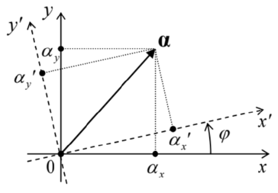
\(\newcommand{\avec}{\mathbf a}\) \(\newcommand{\bvec}{\mathbf b}\) \(\newcommand{\cvec}{\mathbf c}\) \(\newcommand{\dvec}{\mathbf d}\) \(\newcommand{\dtil}{\widetilde{\mathbf d}}\) \(\newcommand{\evec}{\mathbf e}\) \(\newcommand{\fvec}{\mathbf f}\) \(\newcommand{\nvec}{\mathbf n}\) \(\newcommand{\pvec}{\mathbf p}\) \(\newcommand{\qvec}{\mathbf q}\) \(\newcommand{\svec}{\mathbf s}\) \(\newcommand{\tvec}{\mathbf t}\) \(\newcommand{\uvec}{\mathbf u}\) \(\newcommand{\vvec}{\mathbf v}\) \(\newcommand{\wvec}{\mathbf w}\) \(\newcommand{\xvec}{\mathbf x}\) \(\newcommand{\yvec}{\mathbf y}\) \(\newcommand{\zvec}{\mathbf z}\) \(\newcommand{\rvec}{\mathbf r}\) \(\newcommand{\mvec}{\mathbf m}\) \(\newcommand{\zerovec}{\mathbf 0}\) \(\newcommand{\onevec}{\mathbf 1}\) \(\newcommand{\real}{\mathbb R}\) \(\newcommand{\twovec}[2]{\left[\begin{array}{r}#1 \\ #2 \end{array}\right]}\) \(\newcommand{\ctwovec}[2]{\left[\begin{array}{c}#1 \\ #2 \end{array}\right]}\) \(\newcommand{\threevec}[3]{\left[\begin{array}{r}#1 \\ #2 \\ #3 \end{array}\right]}\) \(\newcommand{\cthreevec}[3]{\left[\begin{array}{c}#1 \\ #2 \\ #3 \end{array}\right]}\) \(\newcommand{\fourvec}[4]{\left[\begin{array}{r}#1 \\ #2 \\ #3 \\ #4 \end{array}\right]}\) \(\newcommand{\cfourvec}[4]{\left[\begin{array}{c}#1 \\ #2 \\ #3 \\ #4 \end{array}\right]}\) \(\newcommand{\fivevec}[5]{\left[\begin{array}{r}#1 \\ #2 \\ #3 \\ #4 \\ #5 \\ \end{array}\right]}\) \(\newcommand{\cfivevec}[5]{\left[\begin{array}{c}#1 \\ #2 \\ #3 \\ #4 \\ #5 \\ \end{array}\right]}\) \(\newcommand{\mattwo}[4]{\left[\begin{array}{rr}#1 \amp #2 \\ #3 \amp #4 \\ \end{array}\right]}\) \(\newcommand{\laspan}[1]{\text{Span}\{#1\}}\) \(\newcommand{\bcal}{\cal B}\) \(\newcommand{\ccal}{\cal C}\) \(\newcommand{\scal}{\cal S}\) \(\newcommand{\wcal}{\cal W}\) \(\newcommand{\ecal}{\cal E}\) \(\newcommand{\coords}[2]{\left\{#1\right\}_{#2}}\) \(\newcommand{\gray}[1]{\color{gray}{#1}}\) \(\newcommand{\lgray}[1]{\color{lightgray}{#1}}\) \(\newcommand{\rank}{\operatorname{rank}}\) \(\newcommand{\row}{\text{Row}}\) \(\newcommand{\col}{\text{Col}}\) \(\renewcommand{\row}{\text{Row}}\) \(\newcommand{\nul}{\text{Nul}}\) \(\newcommand{\var}{\text{Var}}\) \(\newcommand{\corr}{\text{corr}}\) \(\newcommand{\len}[1]{\left|#1\right|}\) \(\newcommand{\bbar}{\overline{\bvec}}\) \(\newcommand{\bhat}{\widehat{\bvec}}\) \(\newcommand{\bperp}{\bvec^\perp}\) \(\newcommand{\xhat}{\widehat{\xvec}}\) \(\newcommand{\vhat}{\widehat{\vvec}}\) \(\newcommand{\uhat}{\widehat{\uvec}}\) \(\newcommand{\what}{\widehat{\wvec}}\) \(\newcommand{\Sighat}{\widehat{\Sigma}}\) \(\newcommand{\lt}{<}\) \(\newcommand{\gt}{>}\) \(\newcommand{\amp}{&}\) \(\definecolor{fillinmathshade}{gray}{0.9}\)From the discussion of the last section, it may look that the matrix language is fully similar to, and in many instances more convenient than the general bra-ket formalism. In particular, Eqs. (54)-(55) and (63)-(64) show that any part of any bra-ket expression may be directly mapped on the similar matrix expression, with the only slight inconvenience of using not only columns but also rows (with their elements complex-conjugated), for state vector representation. This invites the question: why do we need the bra-ket language at all? The answer is that the elements of the matrices depend on the particular choice of the basis set, very much like the Cartesian components of a usual geometric vector depend on the particular choice of reference frame orientation (Fig. 4), and very frequently, at problem solution, it is convenient to use two or more different basis sets for the same system. (Just a bit more patience numerous examples will follow soon.)
With this motivation, let us explore what happens at the transform from one basis, \(\{u\}\), to another one, \(\{v\}\) - both full and orthonormal. First of all, let us prove that for each such pair of bases, and an arbitrary numbering of the states of each base, there exists such an operator \(\hat{U}\) that, first,
Unitary operator:
\[\ \left|\nu_{j}\right\rangle=\hat{U}\left|u_{j}\right\rangle,\]
and, second,
\[\ \hat{U} \hat{U}^{\dagger}=\hat{U}^{\dagger} \hat{U}=\hat{I}.\]
(Due to the last property,16 \(\ \hat{U}\) is called a unitary operator, and Eq. (75), a unitary transformation.)
A very simple proof of both statements may be achieved by construction. Indeed, let us take
Unitary operator: construction
\[\ \hat{U} \equiv \sum_{j^{\prime}}\left|\nu_{j^{\prime}}\right\rangle\left\langle u_{j^{\prime}}\right|,\] - an evident generalization of Eq. (44). Then, using Eq. (38), we obtain \[\ \hat{U}\left|u_{j}\right\rangle=\sum_{j^{\prime}}\left|\nu_{j^{\prime}}\right\rangle\left\langle u_{j^{\prime}} \mid u_{j}\right\rangle=\sum_{j^{\prime}}\left|\nu_{j^{\prime}}\right\rangle \delta_{j j}=\left|\nu_{j}\right\rangle,\] so that Eq. (75) has been proved. Now, applying Eq. (31) to each term of the sum (77), we get
Conjugate unitary operator \[\ \hat{U}^{\dagger} \equiv \sum_{j^{\prime}}\left|u_{j^{\prime}}\right\rangle\left\langle \nu_{j^{\prime}}\right|,\] so that \[\hat{U} \hat{U}^{\dagger}=\sum_{j, j^{\prime}}\left|v_{j}\right\rangle\left\langle u_{j} \mid u_{j^{\prime}}\right\rangle\left\langle v_{j^{\prime}}\left|=\sum_{j, j^{\prime}}\right| v_{j}\right\rangle \delta_{i j^{\prime}}\left\langle v_{j^{\prime}}\left|=\sum_{j}\right| v_{j}\right\rangle\left\langle v_{j}\right|\] But according to the closure relation (44), the last expression is just the identity operator, so that one of Eqs. (76) has been proved. (The proof of the second equality is absolutely similar.) As a by-product of our proof, we have also got another important expression - Eq. (79). It implies, in particular, that while, according to Eq. (75), the operator \(\hat{U}\) performs the transform from the "old" basis \(u_{j}\) to the "new" basis \(v_{j}\), its Hermitian adjoint \(\hat{U}^{\dagger}\) performs the reciprocal transform: \[\hat{U}^{\dagger}\left|v_{j}\right\rangle=\sum_{j^{\prime}}\left|u_{j^{\prime}}\right\rangle \delta_{j j}=\left|u_{j}\right\rangle\] Now let us see how do the matrix elements of the unitary transform operators look like. Generally, as was discussed above, the operator’s elements may depend on the basis we calculate them in, so let us be specific - at least initially. For example, let us calculate the desired matrix elements \(U_{j j}\) ’ in the "old" basis \(\{u\}\), using Eq. (77): \[\left.U_{i j^{\prime}}\right|_{\text {in } u} \equiv\left\langle u_{j}|\hat{U}| u_{j^{\prime}}\right\rangle=\left\langle u_{j}\left(\sum_{j^{\prime \prime}}\left|v_{j^{\prime}}\right\rangle\left\langle u_{j^{\prime \prime}}\right|\right) \mid u_{j^{\prime}}\right\rangle=\left\langle u_{j}\left|\sum_{j^{\prime \prime}}\right| v_{j^{\prime \prime}}\right\rangle \delta_{j^{\prime \prime \prime}}=\left\langle u_{j} \mid v_{j^{\prime}}\right\rangle .\] Now performing a similar calculation in the "new" basis \(\{v\}\), we get \[U_{i j^{\prime} \mid \text { in } v} \equiv\left\langle v_{j}|\hat{U}| v_{j^{\prime}}\right\rangle=\left\langle v_{j}\left|\left(\sum_{j^{\prime \prime}}\left|v_{j^{\prime \prime}}\right\rangle\left\langle u_{j^{\prime \prime}}\right|\right)\right| v_{j^{\prime}}\right\rangle=\sum_{j^{\prime \prime}} \delta_{j j^{\prime \prime}}\left\langle u_{j^{\prime \prime}} \| v_{j^{\prime}}\right\rangle=\left\langle u_{j} \mid v_{j^{\prime}}\right\rangle .\] Surprisingly, the result is the same! This is of course true for the Hermitian conjugate (79) as well: \[\left.U_{i j^{\prime}}^{\dagger}\right|_{\text {in } u}=\left.U_{i j^{\prime}}^{\dagger}\right|_{\text {in } v}=\left\langle v_{j} \mid u_{j^{\prime}}\right\rangle .\] These expressions may be used, first of all, to rewrite Eq. (75) in a more direct form. Applying the first of Eqs. (41) to any state \(v_{j}\) ’ of the "new" basis, and then Eq. (82), we get \[\left|v_{j^{\prime}}\right\rangle=\sum_{j}\left|u_{j}\right\rangle\left\langle u_{j} \mid v_{j^{\prime}}\right\rangle=\sum_{j} U_{j j^{\prime}}\left|u_{j}\right\rangle .\] Similarly, the reciprocal transform is \[\left|u_{j^{\prime}}\right\rangle=\sum_{j}\left|v_{j}\right\rangle\left\langle v_{j} \mid u_{j^{\prime}}\right\rangle=\sum_{j} U_{i j^{\prime}}^{\dagger}\left|v_{j}\right\rangle .\] These formulas are very convenient for applications; we will use them already in this section.
Next, we may use Eqs. (83)-(84) to express the effect of the unitary transform on the expansion coefficients \(\alpha_{j}\) of the vectors of an arbitrary state \(\alpha\), defined by Eq. (37). As a reminder, in the "old" basis \(\{u\}\) they are given by Eqs. (40). Similarly, in the "new" basis \(\{v\}\), \[\left.\alpha_{j}\right|_{\text {in } v}=\left\langle v_{j} \mid \alpha\right\rangle .\] Again inserting the identity operator in its closure form (44) with the internal index \(j\) ’, and then using Eqs. (84) and (40), we get \[\left.\alpha_{j}\right|_{\text {in } v}=\left\langle v_{j} \mid\left(\sum_{j^{\prime}}\left|u_{j^{\prime}}\right\rangle\left\langle u_{j^{\prime}}\right|\right) \alpha\right\rangle=\sum_{j^{\prime}}\left\langle v_{j} \mid u_{j^{\prime}}\right\rangle\left\langle u_{j^{\prime}} \mid \alpha\right\rangle=\sum_{j^{\prime}} U_{i j^{\prime}}^{\dagger}\left\langle u_{j^{\prime}} \mid \alpha\right\rangle=\left.\sum_{j^{\prime}} U_{i j^{\prime}}^{\dagger} \alpha_{j^{\prime}}\right|_{\text {in } u} .\] The reciprocal transform is performed by matrix elements of the operator \(\hat{U}\) : \[\left.\alpha_{j}\right|_{\operatorname{in} u}=\left.\sum_{j^{\prime}} U_{j j^{\prime}} \alpha_{j^{\prime}}\right|_{\text {in } v} .\] So, if the transform (75) from the "old" basis \(\{u\}\) to the "new" basis \(\{v\}\) is performed by a unitary operator, the change (88) of state vectors components at this transformation requires its Hermitian conjugate. This fact is similar to the transformation of components of a usual vector at coordinate frame rotation. For example, for a \(2 \mathrm{D}\) vector whose actual position in space is fixed (Fig. 4): \[\left(\begin{array}{l} \alpha_{x}{ }^{\prime} \\ \alpha_{y}{ }^{\prime} \end{array}\right)=\left(\begin{array}{cc} \cos \varphi & \sin \varphi \\ -\sin \varphi & \cos \varphi \end{array}\right)\left(\begin{array}{l} \alpha_{x} \\ \alpha_{y} \end{array}\right),\] but the reciprocal transform is performed by a different matrix, which may be obtained from that participating in Eq. (90) by the replacement \(\varphi \rightarrow-\varphi\). This replacement has a clear geometric sense: if the "new" reference frame \(\{x\) ’, \(y\) ’ \(\}\) is obtained from the "old" frame \(\{x, y\}\) by a counterclockwise rotation by angle \(\varphi\), the reciprocal transformation requires angle \(-\varphi\). (In this analogy, the unitary property \((76)\) of the unitary transform operators corresponds to the equality of the determinants of both rotation matrices to 1 .)
Due to the analogy between expressions (88) and (89) on one hand, and our old friend Eq. (62) on the other hand, it is tempting to skip indices in these new results by writing \[|\alpha\rangle_{\text {in } v}=\hat{U}^{\dagger}|\alpha\rangle_{\text {in } u}, \quad|\alpha\rangle_{\text {in } u}=\hat{U}|\alpha\rangle_{\text {in } v} . \quad(\text { SYMBOLIC ONLY! })\] Since the matrix elements of \(\hat{U}\) and \(\hat{U}^{\dagger}\) do not depend on the basis, such language is not too bad and is mnemonically useful. However, since in the bra-ket formalism (or at least its version presented in this course), the state vectors are basis-independent, Eq. (91) has to be treated as a symbolic one, and should not be confused with the strict Eqs. (88)-(89), and with the rigorous basis-independent vector and operator equalities discussed in Sec. 2 .
Now let us use the same trick of identity operator insertion, repeated twice, to find the transformation rule for matrix elements of an arbitrary operator: \[\left.A_{j j^{\prime}}\right|_{\text {in } v} \equiv\left\langle v_{j}|\hat{A}| v_{j^{\prime}}\right\rangle=\left\langle v_{j}\left|\left(\sum_{k}\left|u_{k}\right\rangle\left\langle u_{k}\right|\right) \hat{A}\left(\sum_{k^{\prime}}\left|u_{k^{\prime}}\right\rangle\left\langle u_{k^{\prime}}\right|\right)\right| v_{j^{\prime}}\right\rangle=\left.\sum_{k, k^{\prime}} U_{j k}^{\dagger} A_{k k^{\prime}}\right|_{\text {in } u} U_{k j^{\prime}}\] \[\left.\left.A_{j j^{\prime}}\right|_{\text {in } u} \equiv \sum_{k, k^{\prime}} U_{j k} A_{k k^{\prime}}\right|_{\text {in } \nu} U_{k j^{\prime}}^{\dagger}\] In the spirit of Eq. (91), we may represent these results symbolically as well, in a compact form: \[\left.\hat{A}\right|_{\text {in } v}=\left.\hat{U}^{\dagger} \hat{A}\right|_{\text {in } u} \hat{U},\left.\quad \hat{A}\right|_{\text {in } u}=\left.\hat{U} \hat{A}\right|_{\text {in } v} \hat{U}^{\dagger} . \quad \text { (SYMBOLIC ONLY!) }\] As a sanity check, let us apply Eq. (93) to the identity operator: \[\left.\hat{I}\right|_{\text {in } v}=\left(\hat{U}^{\dagger} \hat{I} \hat{U}\right)_{\text {in } u}=\left(\hat{U}^{\dagger} \hat{U}\right)_{\text {in } u}=\left.\hat{I}\right|_{\text {in } u}\]
- as it should be. One more (strict rather than symbolic) invariant of the basis change is the trace of any operator, defined as the sum of the diagonal terms of its matrix:
\[\operatorname{Tr} \hat{A} \equiv \operatorname{Tr} \mathrm{A} \equiv \sum_{j} A_{j j} .\] The (easy) proof of this fact, using previous relations, is left for the reader’s exercise.
So far, I have implied that both state bases \(\{u\}\) and \(\{v\}\) are known, and the natural question is where does this information come from in quantum mechanics of actual physical systems. To get a partial answer to this question, let us return to Eq. (68), which defines the eigenstates and the eigenvalues of an operator. Let us assume that the eigenstates \(a_{j}\) of a certain operator \(\hat{A}\) form a full and orthonormal set, and calculate the matrix elements of the operator in the basis \(\{a\}\) of these states, at their arbitrary numbering. For that, it is sufficient to inner-multiply both sides of Eq. (68), written for some index \(j\) ’, by the bra-vector of an arbitrary state \(a_{j}\) of the same set: \[\left\langle a_{j}|\hat{A}| a_{j^{\prime}}\right\rangle=\left\langle a_{j}\left|A_{j^{\prime}}\right| a_{j^{\prime}}\right\rangle .\] The left-hand side of this equality is the matrix element \(A_{j j}\) ’ we are looking for, while its right-hand side is just \(A_{j} \cdot \delta_{i j}\) ’. As a result, we see that the matrix is diagonal, with the diagonal consisting of the operator’s eigenvalues: \[A_{i j^{\prime}}=A_{j} \delta_{j j^{\prime}}\] In particular, in the eigenstate basis (but not necessarily in an arbitrary basis!), \(A_{j j}\) means the same as \(A_{j}\). Thus the important problem of finding the eigenvalues and eigenstates of an operator is equivalent to the diagonalization of its matrix, \({ }^{17}\) i.e. finding the basis in which the operator’s matrix acquires the diagonal form \((98)\); then the diagonal elements are the eigenvalues, and the basis itself is the desirable set of eigenstates.
To see how this is done in practice, let us inner-multiply Eq. (68) by a bra-vector of the basis (say, \(\{u\}\) ) in that we have happened to know the matrix elements \(A_{j j}\) ’: \[\left\langle u_{k}|\hat{A}| a_{j}\right\rangle=\left\langle u_{k}\left|A_{j}\right| a_{j}\right\rangle .\] On the left-hand side, we can (as usual :-) insert the identity operator between the operator \(\hat{A}\) and the ket-vector, and then use the closure relation (44) in the same basis \(\{u\}\), while on the right-hand side, we can move the eigenvalue \(A_{j}\) (a \(c\)-number) out of the bracket, and then insert a summation over the same index as in the closure, compensating it with the proper Kronecker delta symbol: \[\left\langle u_{k}\left|\hat{A} \sum_{k^{\prime}}\right| u_{k^{\prime}}\right\rangle\left\langle u_{k^{\prime}} \mid a_{j}\right\rangle=A_{j} \sum_{k^{\prime}}\left\langle u_{k^{\prime}} \mid a_{j}\right\rangle \delta_{k k^{\prime}} .\] Moving out the signs of summation over \(k^{\prime}\), and using the definition (47) of the matrix elements, we get
\[\sum_{k^{\prime}}\left(A_{k k^{\prime}}-A_{j} \delta_{k k^{\prime}}\right)\left\langle u_{k^{\prime}} \mid a_{j}\right\rangle=0 .\] But the set of such equalities, for all \(N\) possible values of the index \(k\), is just a system of linear, homogeneous equations for unknown \(c\)-numbers \(\left\langle u_{k} \mid a_{j}\right\rangle\). According to Eqs. (82)-(84), these numbers are nothing else than the matrix elements \(U_{k^{\prime} j}\) of a unitary matrix providing the required transformation from the initial basis \(\{u\}\) to the basis \(\{a\}\) that diagonalizes the matrix A. This system may be represented in the matrix form: \[\left(\begin{array}{ccc} A_{11}-A_{j} & A_{12} & \ldots \\ A_{21} & A_{22}-A_{j} & \ldots \\ \ldots & \ldots & \ldots \end{array}\right)\left(\begin{array}{c} U_{1 j} \\ U_{2 j} \\ \ldots \end{array}\right)=0\] and the condition of its consistency,
\(\begin{array}{r}\begin{array}{c}\text { Characteristic } \\ \text { equation } \\ \text { for }\end{array} \\ \text { eigenvalues }\end{array} \quad\left|\begin{array}{ccc}A_{11}-A_{j} & A_{12} & \cdots \\ A_{21} & A_{22}-A_{j} & \cdots \\ \ldots & \cdots & \cdots\end{array}\right|=0\),
plays the role of the characteristic equation of the system. This equation has \(N\) roots \(A_{j}-\) the eigenvalues of the operator \(\hat{A}\); after they have been calculated, plugging any of them back into the system (102), we can use it to find \(N\) matrix elements \(U_{k j}(k=1,2, \ldots N)\) corresponding to this particular eigenvalue. However, since the equations (103) are homogeneous, they allow finding \(U_{k j}\) only to a constant multiplier. To ensure their normalization, i.e. enforce the unitary character of the matrix U, we may use the condition that all eigenvectors are normalized (just as the basis vectors are): \[\left\langle a_{j} \mid a_{j}\right\rangle \equiv \sum_{k}\left\langle a_{j} \mid u_{k}\right\rangle\left\langle u_{k} \mid a_{j}\right\rangle \equiv \sum_{k}\left|U_{k j}\right|^{2}=1,\] for each \(j\). This normalization completes the diagonalization. \({ }^{18}\)
Now (at last!) I can give the reader some examples. As a simple but very important case, let us diagonalize each of the operators described (in a certain two-function basis \(\{u\}\), i.e. in two-dimensional Hilbert space) by the so-called Pauli matrices \[\sigma_{x} \equiv\left(\begin{array}{ll} 0 & 1 \\ 1 & 0 \end{array}\right), \quad \sigma_{y} \equiv\left(\begin{array}{cc} 0 & -i \\ i & 0 \end{array}\right), \quad \sigma_{z} \equiv\left(\begin{array}{cc} 1 & 0 \\ 0 & -1 \end{array}\right) .\] Though introduced by a physicist, with a specific purpose to describe electron’s spin, these matrices have a general mathematical significance, because together with the \(2 \times 2\) identity matrix, they provide a full, linearly-independent system - meaning that an arbitrary \(2 \times 2\) matrix may be represented as \[\left(\begin{array}{ll} A_{11} & A_{12} \\ A_{21} & A_{22} \end{array}\right)=b \mathrm{I}+c_{x} \sigma_{x}+c_{y} \sigma_{y}+c_{z} \sigma_{z},\] with a unique set of four \(c\)-number coefficients \(b, c_{x}, c_{y}\), and \(c_{z}\).
Since the matrix \(\sigma_{z}\) is already diagonal, with the evident eigenvalues \(\pm 1\), let us start with diagonalizing the matrix \(\sigma_{x}\). For it, the characteristic equation (103) is evidently \[\left|\begin{array}{cc} -A_{j} & 1 \\ 1 & -A_{j} \end{array}\right|=0, \quad \text { i.e. } A_{j}^{2}-1=0,\] and has two roots, \(A_{1,2}=\pm 1\). (Again, the state numbering is arbitrary!) So the eigenvalues of the matrix \(\sigma_{x}\) are the same as of the matrix \(\sigma_{z}\). (The reader may readily check that the eigenvalues of the matrix \(\sigma_{y}\) are also the same.) However, the eigenvectors of the operators corresponding to these three matrices are different. To find them for \(\sigma_{x}\), let us plug its first eigenvalue, \(A_{1}=+1\), back into equations (101) spelled out for this particular case \(\left(j=1 ; k, k^{\prime}=1,2\right)\) : \[\begin{gathered} -\left\langle u_{1} \mid a_{1}\right\rangle+\left\langle u_{2} \mid a_{1}\right\rangle=0, \\ \left\langle u_{1} \mid a_{1}\right\rangle-\left\langle u_{2} \mid a_{1}\right\rangle=0 . \end{gathered}\] These two equations are compatible (of course, because the used eigenvalue \(A_{1}=+1\) satisfies the characteristic equation), and any of them gives \[\left\langle u_{1} \mid a_{1}\right\rangle=\left\langle u_{2} \mid a_{1}\right\rangle \text {, i.e. } U_{11}=U_{21} \text {. }\] With that, the normalization condition (104) yields \[\left|U_{11}\right|^{2}=\left|U_{21}\right|^{2}=\frac{1}{2} .\] Although the normalization is insensitive to the simultaneous multiplication of \(U_{11}\) and \(U_{21}\) by the same phase factor \(\exp \{i \varphi\}\) with any real \(\varphi\), it is convenient to keep the coefficients real, for example taking \(\varphi\) \(=0\), to \(\mathrm{get}\) \[U_{11}=U_{21}=\frac{1}{\sqrt{2}} .\] Performing an absolutely similar calculation for the second characteristic value, \(A_{2}=-1\), we get \(U_{12}=-U_{22}\), and we may choose the common phase to have \[U_{12}=-U_{22}=\frac{1}{\sqrt{2}},\] so that the whole unitary matrix for diagonalization of the operator corresponding to \(\sigma_{x}\) is \({ }^{19}\) \[\mathrm{U}_{x}=\mathrm{U}_{x}^{\dagger}=\frac{1}{\sqrt{2}}\left(\begin{array}{cc} 1 & 1 \\ 1 & -1 \end{array}\right),\] For what follows, it will be convenient to have this result expressed in the ket-relation form - see Eqs. (85)-(86): \[\left|a_{1}\right\rangle=U_{11}\left|u_{1}\right\rangle+U_{21}\left|u_{2}\right\rangle=\frac{1}{\sqrt{2}}\left(\left|u_{1}\right\rangle+\left|u_{2}\right\rangle\right), \quad\left|a_{2}\right\rangle=U_{12}\left|u_{1}\right\rangle+U_{22}\left|u_{2}\right\rangle=\frac{1}{\sqrt{2}}\left(\left|u_{1}\right\rangle-\left|u_{2}\right\rangle\right),\] \[\left|u_{1}\right\rangle=U_{11}^{\dagger}\left|a_{1}\right\rangle+U_{21}^{\dagger}\left|a_{2}\right\rangle=\frac{1}{\sqrt{2}}\left(\left|a_{1}\right\rangle+\left|a_{2}\right\rangle\right), \quad\left|u_{2}\right\rangle=U_{12}^{\dagger}\left|a_{1}\right\rangle+U_{22}^{\dagger}\left|a_{2}\right\rangle=\frac{1}{\sqrt{2}}\left(\left|a_{1}\right\rangle-\left|a_{2}\right\rangle\right) .\] Now let me show that these results are already sufficient to understand the Stern-Gerlach experiments described in Sec. 1 - but with two additional postulates. The first of them is that the interaction of a particle with the external magnetic field, besides that due to its orbital motion, may be described by the following vector operator of its spin dipole magnetic moment: 20 \[\hat{\mathbf{m}}=\hat{\mathbf{S}},\] where the constant coefficient \(\gamma\), specific for every particle type, is called the gyromagnetic ratio, \({ }^{21}\) and \(\hat{\mathbf{S}}\) is the vector operator of spin, with three Cartesian components: \[\hat{\mathbf{S}}=\mathbf{n}_{x} \hat{S}_{x}+\mathbf{n}_{y} \hat{S}_{y}+\mathbf{n}_{z} \hat{S}_{z}\] Here \(\mathbf{n}_{x, y, z}\) are the usual Cartesian unit vectors in the 3D geometric space (in the quantum-mechanics sense, just \(c\)-numbers, or rather " \(c\)-vectors"), while \(\hat{S}_{x, y, z}\) are the "usual" (scalar) operators.
For the so-called \(\operatorname{spin}-1 / 2\) particles (including the electron), these components may be simply, as \[\hat{S}_{x, y, z}=\frac{\hbar}{2} \hat{\sigma}_{x, y, z}\] Spin-1/2
operator expressed via those of the Pauli vector operator \(\hat{\boldsymbol{\sigma}} \equiv \mathbf{n}_{x} \hat{\sigma}_{x}+\mathbf{n}_{y} \hat{\sigma}_{y}+\mathbf{n}_{z} \hat{\sigma}_{z}\), so that we may also write \[\hat{\mathbf{S}}=\frac{\hbar}{2} \hat{\boldsymbol{\sigma}}\] In turn, in the so-called \(z\)-basis, each Cartesian component of the latter operator is just the corresponding Pauli matrix (105), so that it may be also convenient to use the following 3D vector of these matrices: \[\boldsymbol{\sigma} \equiv \mathbf{n}_{x} \sigma_{x}+\mathbf{n}_{y} \sigma_{y}+\mathbf{n}_{z} \sigma_{z} \equiv\left(\begin{array}{cc} \mathbf{n}_{z} & \mathbf{n}_{x}-i \mathbf{n}_{y} \\ \mathbf{n}_{x}+i \mathbf{n}_{y} & -\mathbf{n}_{z} \end{array}\right)\] The \(z\)-basis, in which such matrix representation of \(\hat{\boldsymbol{\sigma}}\) is valid, is defined as an orthonormal basis of certain two states, commonly denoted \(\uparrow\) an \(\downarrow\), in that the matrix of the operator \(\hat{\sigma}_{z}\) is diagonal, with eigenvalues, respectively, \(+1\) and \(-1\), and hence the matrix \(S_{z} \equiv(\hbar / 2) \sigma_{z}\) of \(\hat{S}_{z}\) is also diagonal, with the eigenvalues \(+\hbar / 2\) and \(-\hbar / 2\). Note that we do not "understand" what exactly the states \(\uparrow\) and \(\downarrow\) are, \({ }^{22}\) but loosely associate them with some internal rotation of a spin- \(1 / 2\) particle about the \(z\)-axis, with either positive or negative angular momentum component \(S_{z}\). However, attempts to use such classical interpretation for quantitative predictions runs into fundamental difficulties - see Sec. 6 below.
The second necessary postulate describes the general relation between the bra-ket formalism and experiment. Namely, in quantum mechanics, each real observable \(A\) is represented by a Hermitian operator \(\hat{A}=\hat{A}^{\dagger}\), and the result of its measurement, \({ }^{23}\) in a quantum state \(\alpha\) described by a linear superposition of the eigenstates \(a_{j}\) of the operator, \[|\alpha\rangle=\sum_{j} \alpha_{j}\left|a_{j}\right\rangle, \quad \text { with } \alpha_{j}=\left\langle a_{j} \mid \alpha\right\rangle,\] may be only one of the corresponding eigenvalues \(A_{j} .{ }^{24}\) Specifically, if the ket (118) and all eigenkets \(\left|a_{j}\right\rangle\) are normalized to 1 , \[\langle\alpha \mid \alpha\rangle=1, \quad\left\langle a_{j} \mid a_{j}\right\rangle=1,\] then the probability of a certain measurement outcome \(A_{j}\) is \({ }^{25}\) \[W_{j}=\left|\alpha_{j}\right|^{2} \equiv \alpha_{j}^{*} \alpha_{j} \equiv\left\langle\alpha \mid a_{j}\right\rangle\left\langle a_{j} \mid \alpha\right\rangle,\] This relation is evidently a generalization of Eq. (1.22) in wave mechanics. As a sanity check, let us assume that the set of the eigenstates \(a_{j}\) is full, and calculate the sum of the probabilities to find the system in one of these states: \[\sum_{j} W_{j}=\sum_{j}\left\langle\alpha \mid a_{j}\right\rangle\left\langle a_{j} \mid \alpha\right\rangle=\langle\alpha|\hat{I}| \alpha\rangle=1 .\] Now returning to the Stern-Gerlach experiment, conceptually the description of the first \((z-\) oriented) experiment shown in Fig. 1 is the hardest for us, because the statistical ensemble describing the unpolarized electron beam at its input is mixed ("incoherent"), and cannot be described by a pure ("coherent") superposition of the type (6) that have been the subject of our studies so far. (We will discuss such mixed ensembles in Chapter 7.) However, it is intuitively clear that its results are compatible with the description of the two output beams as sets of electrons in the pure states \(\uparrow\) and \(\downarrow\), respectively. The absorber following that first stage (Fig. 2) just takes all spin-down electrons out of the picture, producing an output beam of polarized electrons in the definite \(\uparrow\) state. For such a beam, the probabilities (120) are \(W_{\uparrow}=1\) and \(W_{\downarrow}=0\). This is certainly compatible with the result of the "control" experiment shown on the bottom panel of Fig. 2: the repeated SG \((z)\) stage does not split such a beam, keeping the probabilities the same.
Now let us discuss the double Stern-Gerlach experiment shown on the top panel of Fig. 2. For that, let us represent the \(z\)-polarized beam in another basis - of the two states (I will denote them as \(\rightarrow\) and \(\leftarrow)\) in that, by definition, the matrix \(S_{x}\) is diagonal. But this is exactly the set we called \(a_{1,2}\) in the \(\sigma_{x}\) matrix diagonalization problem solved above. On the other hand, the states \(\uparrow\) and \(\downarrow\) are exactly what we called \(u_{1,2}\) in that problem, because in this basis, we know matrix \(\sigma\) explicitly - see Eq. (117). Hence, in the application to the electron spin problem, we may rewrite Eqs. (114) as \[\begin{aligned} &|\rightarrow\rangle=\frac{1}{\sqrt{2}}(|\uparrow\rangle+|\downarrow\rangle), \quad|\leftarrow\rangle=\frac{1}{\sqrt{2}}(|\uparrow\rangle-|\downarrow\rangle), \\ &|\uparrow\rangle=\frac{1}{\sqrt{2}}(|\rightarrow\rangle+|\leftarrow\rangle), \quad|\downarrow\rangle=\frac{1}{\sqrt{2}}(|\rightarrow\rangle-|\leftarrow\rangle), \end{aligned}\] Currently for us the first of Eqs. (123) is most important, because it shows that the quantum state of electrons entering the SG \((x)\) stage may be represented as a coherent superposition of electrons with \(S_{x}=+\hbar / 2\) and \(S_{x}=-\hbar / 2\). Notice that the beams have equal probability amplitude moduli, so that according to Eq. (122), the split beams \(\rightarrow\) and \(\leftarrow\) have equal intensities, in accordance with experimental results. (The minus sign before the second ket-vector is of no consequence here, but it may have an impact on outcomes of other experiments - for example, if coherently split beams are brought together again.)
Now, let us discuss the most mysterious (from the classical point of view) multi-stage SG experiment shown on the middle panel of Fig. 2. After the second absorber has taken out all electrons in, say, the \(\leftarrow\) state, the remaining electrons, all in the state \(\rightarrow\), are passed to the final, SG \((z)\), stage. But according to the first of Eqs. (122), this state may be represented as a (coherent) linear superposition of the \(\uparrow\) and \(\downarrow\) states, with equal probability amplitudes. The final stage separates electrons in these two states into separate beams, with equal probabilities \(W_{\uparrow}=W_{\downarrow}=1 / 2\) to find an electron in each of them, thus explaining the experimental results.
To conclude our discussion of the multistage Stern-Gerlach experiment, let me note that though it cannot be explained in terms of wave mechanics (which operates with scalar de Broglie waves), it has an analogy in classical theories of vector fields, such as the classical electrodynamics. Indeed, let a plane electromagnetic wave propagate normally to the plane of the drawing in Fig. 5, and pass through the linear polarizer \(1 .\)
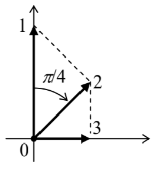 Fig. 4.5. A light polarization sequence similar to the three-stage Stern-Gerlach experiment shown on the middle panel of Fig. \(2 .\)
Similarly to the output of the initial SG \((z)\) stages (including the absorbers) shown in Fig. 2, the output wave is linearly polarized in one direction - the vertical direction in Fig. 5. Now its electric field vector has no horizontal component \(-\) as may be revealed by the wave’s full absorption in a perpendicular polarizer 3 . However, let us pass the wave through polarizer 2 first. In this case, the output wave does acquire a horizontal component, as can be, again, revealed by passing it through polarizer 3 . If the angles between the polarization directions 1 and 2 , and between 2 and 3 , are both equal to \(\pi / 4\), each polarizer reduces the wave amplitude by a factor of \(\sqrt{2}\), and hence the intensity by a factor of 2, exactly like in the multistage SG experiment, with the polarizer 2 playing the role of the SG \((x)\) stage. The "only" difference is that the necessary angle is \(\pi / 4\), rather than by \(\pi / 2\) for the SternGerlach experiment. In quantum electrodynamics (see Chapter 9 below), which confirms classical predictions for this experiment, this difference may be interpreted by that between the integer spin of electromagnetic field quanta (photons) and the half-integer spin of electrons.
\({ }^{16}\) An alternative way to express Eq. (76) is to write \(\hat{U}^{\dagger}=\hat{U}^{-1}\), but I will try to avoid this language.
\({ }^{17}\) Note that the expression "matrix diagonalization" is a very common but dangerous jargon. (Formally, a matrix is just a matrix, an ordered set of \(c\)-numbers, and cannot be "diagonalized".) It is OK to use this jargon if you remember clearly what it actually means - see the definition above.
\({ }^{18}\) A possible slight complication here is that the characteristic equation may give equal eigenvalues for certain groups of different eigenvectors. In such cases, the requirement of the mutual orthogonality of these degenerate states should be additionally enforced.
\({ }^{19}\) Note that though this particular unitary matrix is Hermitian, this is not true for an arbitrary choice of phases \(\varphi\).
\({ }^{20}\) This was the key point in the electron spin’s description, developed by W. Pauli in 1925-1927.
\({ }^{21}\) For the electron, with its negative charge \(q=-e\), the gyromagnetic ratio is negative: \(\gamma_{\mathrm{e}}=-g_{\mathrm{e}} e / 2 m_{\mathrm{e}}\), where \(g_{\mathrm{e}} \approx 2\) is the dimensionless \(g\)-factor. Due to quantum-electrodynamic (relativistic) effects, this \(g\)-factor is slightly higher than \(2: g_{\mathrm{e}}=2(1+\alpha / 2 \pi+\ldots) \approx 2.002319304 \ldots\), where \(\alpha \equiv e^{2} / 4 \pi \varepsilon_{\mathrm{o}} \hbar c \equiv\left(E_{\mathrm{H}} / m_{\mathrm{e}} c^{2}\right)^{1 / 2} \approx 1 / 137\) is the so-called fine structure constant. (The origin of its name will be clear from the discussion in Sec. 6.3.)
\({ }^{22}\) If you think about it, the word "understand" typically means that we can express a new, more complex notion in terms of those discussed earlier and considered "known". In our current case, we cannot describe the spin states by some wavefunction \(\psi(\mathbf{r})\), or any other mathematical notion discussed in the previous three chapters. The braket formalism has been invented exactly to enable mathematical analyses of such "new" quantum states we do not initially "understand". Gradually we get accustomed to these notions, and eventually, as we know more and more about their properties, start treating them as "known" ones.
\({ }^{23}\) Here again, just like in Sec. 1.2, the statement implies the abstract notion of "ideal experiments", deferring the discussion of real (physical) measurements until Chapter 10 .
\({ }^{24}\) As a reminder, at the end of Sec. 3 we have already proved that such eigenstates corresponding to different values \(A_{j}\) are orthogonal. If any of these values is degenerate, i.e. corresponds to several different eigenstates, they should be also selected orthogonal, in order for Eq. (118) to be valid.
\({ }^{25}\) This key relation, in particular, explains the most common term for the (generally, complex) coefficients \(\alpha_{j}\), the probability amplitudes.