
2.5: Fermi's Golden Rule in a 1D Resonance Model


- Last updated
- May 1, 2021
- Save as PDF

( \newcommand{\kernel}{\mathrm{null}\,}\)
Fermi’s golden rule can be used to study a wide variety of quantum systems, and we will see examples of its usefulness in subsequent chapters. In this section, we will apply it to the simple 1D model from Section 2.2, and evaluate how well it works. The model potential is
V(x)=V0(x)+V1(x),whereV0(x)=−UΘ(a−|x|),V1(x)=VbΘ(b−|x|),0<U<Vb.
The potential well V0 supports one or more bound states. For simplicity, we focus on the ground state, whose energy E0 lies in the range [−U,0]. Once V1 is introduced, this will turn into the lowest quasi-bound state, with resonance energy Eres≈E0+Vb>0.
When the potential consists only of V0, the ground state wavefunction can be obtained by solving the Schrödinger wave equation for the boundary condition φ(x)→0 as |x|→∞. It has the form
φ(x)={Acos(qx),|x|<aBexp(−η|x|),|x|≥a,
where A and B are constants to be determined, and
q=√2mℏ2(E0+U),η=√2mℏ2|E0|.
By matching both φ(x) and dφ/dx across the x=a interface, we can derive a transcendental equation for E0, which can be solved numerically. Once we know E0, we also know q and η. We can then relate A and B by matching φ(x) across the x=a interface:
A=Bexp(−ηa)cos(qa).
Moreover, the wavefunction must be normalized to unity:
1=A2∫a−acos2(qx)+2B2∫∞adxexp(−2ηx)=A2(a+sin(2qa)2q)+B2exp(−2ηa)η.
Putting the last two equations together yields
B2=exp(2ηa)a[1+sin(2qa)/2qacos2(qa)+1ηa]−1.
We now wish to compute the transition amplitude
⟨ψk|ˆV1|φ⟩=∫∞−∞dxψ∗k(x)V1(x)φ(x)=Vb∫b−bdxψ∗k(x)φ(x),
where ψk(x) is the wavefunction of a free state for the system with potential V0(x), which is labeled by some continuous index k. We can use a trick to avoid calculating the exact form of ψk(x). Because ψk(x) and φ(x) must be orthogonal,
∫b−bdxψ∗k(x)φ(x)=−∫|x|>adxψ∗k(x)φ(x).
When evaluating the free states outside the potential well, we can approximate them as the free states of the particle without the potential well, i.e., simple plane waves:
ψk(x)=1√2πeikx,k∈R,|x|>a.
We likewise approximate their energies by Ek≈ℏ2k2/2m. Plugging ψk(x) into the formula for the transition amplitude, and performing the necessary integrals, yields
⟨ψk|ˆV1|φ⟩=−B√2πℏ22m[ηcos(kb)−ksin(kb)]exp(−ηb).
Within Fermi’s golden rule, we must use a value of k such that
Ek=Eres≈E0+Vb⇒k≈√2mℏ2(E0+Vb).
The next thing that we need to calculate is the density of free states. This can be done by once again taking Ek≈ℏ2k2/2m, and performing a change of variables:
D(E)=∫∞−∞dkδ(E−ℏ2k22m)=2⋅∫∞0dE′dkdE′δ(E−E′)=√2mℏ2E.
Note the factor of 2 on the second line; it is there because there is both a positive and a negative value of k for each E.
Having obtained expressions for the transition amplitude and the density of states, we just have to plug them into Fermi’s golden rule to obtain the decay rate κ. The figure below shows how κ varies with the barrier thickness b−a, with all other model parameters fixed (U=20,Vb=30,a=1):
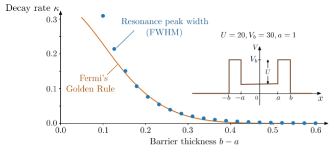
For comparison, the figure also plots the width of the resonant scattering peak, which according to our preceding discussion is supposed to be equal to κ. To obtain these values, we use the transfer matrix method to compute the E-dependent transmittance for particles incident on one side of the potential (see Appendix B). The transmittance is peaked near Eres, and the full-width at half-maximum (see Section 2.3) is estimated numerically. The results are shown as blue dots in the figure.
We see that Fermi’s golden rule generally agrees well with the results from the transfer matrix method. There is some discrepancy, notably when the barrier is thin. Remember that Fermi’s golden rule relies on the approximation that the quasi-bound state is strongly confined (i.e., having ⟨φ|G|φ⟩ be large in the derivations of Sections 2.3 and 2.4). Moreover, we have approximated the free states |ψk⟩ using the plane wave states in the absence of any potential, which is an assumption commonly employed when using Fermi’s golden rule.