11.4: Scattering in one dimension - Square Well

The square well potential has $V (x < 0) = V (x > a) = 0; V (0 < x < a) = V_0$. As with the step function, we can write the wavefunction as a plane wave in each of the three regions.

$$\Phi (x < 0) = A \text{ exp}(ikx) + B \text{ exp}(−ikx) \nonumber$$

$$\Phi (0 < x < a) = F \text{ exp}(ik0x) + G \text{ exp}(−ik0x) \nonumber$$

$$\Phi (x > a) = C \text{ exp}(ikx) + D \text{ exp}(−ikx) \nonumber$$

Once again there is no wave coming back from $x = \infty (D = 0)$.

There are now four boundary conditions from continuity of the wave function and its derivative at x=0 and x=a. The solving of four equations in four unknowns is straightforward but tedious. Eventually one can obtain ratios for reflected and transmitted flux:

$$B/A = \frac{(k^2 − k^{'2} )(1 − e^{2ik'a} )}{(k + k' )^2 − (k − k' )^2 e^{2ik'a}} \nonumber$$

$$C/A = \frac{4kk' e^{i(k' − k)a}}{(k + k' )^2 − (k − k' )^2 e^{2ik'a}} \nonumber$$

where $k^2 = 2mE/\hbar^2$ and $k^{'2} = 2m(E − V_0)/\hbar^2$. Since the wavenumber is the same on both sides of the barrier, the reflection and transmission coefficients are just:

$$|B/A|^2 = \left[ 1 + \frac{4k^2 k^{'2}}{(k^2 − k^{'2} )^2 \sin^2 k' a} \right]^{−1} = \left[ 1 + \frac{4E(E − V_0)}{V^2_0 \sin^2 k' a} \right]^{−1} \nonumber$$

$$|C/A|^2 = \left[ 1 + \frac{(k^2 − k^{'2} )^2 \sin^2 k' a}{4k^2 k^{'2}} \right]^{−1} = \left[ 1 + \frac{V^2_0 \sin^2 k' a}{4E(E − V_0)} \right]^{-1} \nonumber$$

We get complete transmission when $k' a = n\pi$, i.e. when an exact number of half waves fit in the well.

Assuming that $E > V_0$. Looking at the limits of this, we see that as $E \rightarrow V_0$ then $\sin^2 (k' a) \rightarrow k' a$ and the transmission coefficient

$$|C/A|^2 \rightarrow \left[ 1 + \frac{mV_0a^2}{2\hbar^2} \right]^{-1} \nonumber$$

As the incoming particle energy is increased, the transmission oscillates between $\left[1 + \frac{V^2_0}{4E(E−V_0)} \right]^{−1}$ and 1 at $k' a = n\pi$. The lower limit itself increases to 1 as E increases.

For the tunnelling case where $E < V_0$ we can use these solutions for B/A and C/A, except that $k'$ is now imaginary. This gives

$$|C/A|^2 = \left[ 1 + \frac{4E(E − V_0)}{V^2_0 \sinh^2 |k' |a} \right]^{−1} \nonumber$$

which decreases monotonically with decreasing E. Thus a small change in $V_0$ can give a large change in $|C/A|^2$. This is the principle on which the transistor and the tunnelling electron microscope are based.

Note that the transmitted wave $\Phi (x > a) = C \text{ exp}(ikx)$, differs from the incident wave only by a phase - it has the same wavevector. Thus the only effect of the potential on the transmitted particles is to change their phase, an idea we shall meet again.

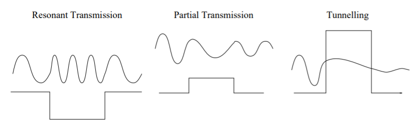
Figure $\PageIndex{1}$: Forward moving wavefunctions passing a square well potential