
2.5: Relativistic Properties of Lorentz Geometry (Part 2)


- Last updated
- Mar 5, 2022
- Save as PDF

( \newcommand{\kernel}{\mathrm{null}\,}\)
Example 8
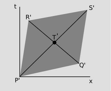
Let the intersection of the parallelogram’s two diagonals be T in the original (rest) frame, and T' in the Lorentz-boosted frame. An observer at T in the original frame simultaneously detects the passing by of the two flashes of light emitted at P and Q, and since she is positioned at the midpoint of the diagram in space, she infers that P and Q were simultaneous. Since the arrival of both flashes of light at the same point in spacetime is a concrete event, an observer in the Lorentz-boosted frame must agree on their simultaneous arrival. (Simultaneity is well defined as long as no spatial separation is involved.) But the distances traveled by the two flashes in the boosted frame are unequal, and since the speed of light is the same in all cases, the boosted observer infers that they were not emitted simultaneously.
Example 9
A different kind of symmetry is the symmetry between observers. If observer A says observer B’s time is slow, shouldn’t B say that A’s time is fast? This is what would happen if B took a pill that slowed down all his thought processes: to him, the rest of the world would seem faster than normal. But this can’t be correct for Lorentz boosts, because it would introduce an asymmetry between observers. There is no preferred, “correct” frame corresponding to the observer who didn’t take a pill; either observer can correctly consider himself to be the one who is at rest. It may seem paradoxical that each observer could think that the other was the slow one, but the paradox evaporates when we consider the methods available to A and B for resolving the controversy. They can either (1) send signals back and forth, or (2) get together and compare clocks in person. Signaling doesn’t establish one observer as correct and one as incorrect, because as we’ll see in the following section, there is a limit to the speed of propagation of signals; either observer ends up being able to explain the other observer’s observations by taking into account the finite and changing time required for signals to propagate. Meeting in person requires one or both observers to accelerate, as in the original story of Alice and Betty, and then we are no longer dealing with pure Lorentz frames, which are described by nonaccelerating observers.
Example 10: Einstein’s goof
Einstein’s original 1905 paper on special relativity, reproduced in Appendix A, contains a famous incorrect prediction, that “a spring-clock at the equator must go more slowly, by a very small amount, than a precisely similar clock situated at one of the poles under otherwise identical conditions”. This was a reasonable prediction at the time, but we now know that it was incorrect because it neglected gravitational time dilation. In the description of the Hafele-Keating experiment using atomic clocks aboard airplanes, we saw that both gravity and motion had effects on the rate of flow of time. Earlier we found based on the equivalence principle that the gravitational redshift of an electromagnetic wave is ΔEE=Δϕ (where c = 1 and ϕ is the gravitational potential gy), and that this could also be interpreted as a gravitational time dilation Δtt=Δϕ.
The clock at the equator suffers a kinematic time dilation that would tend to cause it to run more slowly than the one at the pole. However, the earth is not a sphere, so the two clocks are at different distances from the earth’s center, and the field they inhabit is also not the simple field of a sphere. This suggests that there may be an additional gravitational effect due to Δϕ≠0. Expanding the Lorentz gamma factor in a Taylor series, we find that the kinematic effect amounts to Δtt=γ−1≈v22. The mismatch in rates between the two clocks is
Δtt≈12v2−Δϕ,
where Δϕ=ϕequator−ϕpole, and a factor of frac1c2 on the right is suppressed because c = 1. But this expression for Δtt vanishes, because the surface of the earth’s oceans is in equilibrium, and therefore a mass of water m can be brought from the north pole to the equator, with the change in potential energy −mΔϕ being exactly sufficient to supply the necessary kinetic energy (12)mv2. We therefore find that a change of latitude should have no effect on the rate of a clock, provided that it remains at sea level.
This has been verified experimentally by Alley et al.9 Alley’s group flew atomic clocks from Washington, DC to Thule, Greenland, left them there for four days, and brought them back. The difference between the clocks that went to Greenland and other clocks that stayed in Washington was 38 ± 5 ns, which was consistent with the 35 ± 2 ns effect predicted purely based on kinematic and gravitational time dilation while the planes were in the air. If Einstein’s 1905 prediction had been correct, then there would have been an additional difference of 224 ns due to the difference in latitude.
The perfect cancellation of kinematic and gravitational effects is not as fortuitous as it might seem; this is discussed in example 18.
9 C.O. Alley, et al., in NASA Goddard Space Flight Center, Proc. of the 13th Ann. Precise Time and Time Interval (PTTI) Appl. and Planning Meeting, p. 687-724, 1981, available online at http://www.pttimeeting.org/archivemeetings/index9.html
Example 11: GPS
In the GPS system, as in example 10, both gravitational and kinematic time dilation must be considered. Let’s determine the directions and relative strengths of the two effects in the case of a GPS satellite.
A radio photon emitted by a GPS satellite gains energy as it falls to the earth’s surface, so its energy and frequency are increased by this effect. The observer on the ground, after accounting for all non-relativistic effects such as Doppler shifts and the Sagnac effect, would interpret the frequency shift by saying that time aboard the satellite was flowing more quickly than on the ground.
However, the satellite is also moving at orbital speeds, so there is a Lorentz time dilation effect. According to the observer on earth, this causes time aboard the satellite to flow more slowly than on the ground.
We can therefore see that the two effects are of opposite sign. Which is stronger?
For a satellite in low earth orbit, we would have fracv2r=g, where r is only slightly greater than the radius of the earth. The relative effect on the flow of time is γ−1≈v22=gr2. The gravitational effect, approximating g as a constant, is −gy, where y is the satellite’s altitude above the earth. For such a satellite, the gravitational effect is down by a factor of 2yr, so the Lorentz time dilation dominates.
GPS satellites, however, are not in low earth orbit. They orbit at an altitude of about 20,200 km, which is quite a bit greater than the radius of the earth. We therefore expect the gravitational effect to dominate. To confirm this, we need to generalize the equation Δtt=Δϕ (with c = 1) from example 10 to the case where g is not a constant. Integrating the equation dtt=dϕ, we find that the time dilation factor is equal to eΔϕ. When Δϕ is small, eΔϕ≈1+Δϕ, and we have a relative effect equal to Δϕ. The total effect for a GPS satellite is thus (inserting factors of c for calculation with SI units, and using positive signs for blueshifts)
1c2(+Δϕ−v22)=5.2×10⁻¹⁰−0.9×10⁻¹⁰,
where the first term is gravitational and the second kinematic. A more detailed analysis includes various time-varying effects, but this is the constant part. For this reason, the atomic clocks aboard the satellites are set to a frequency of 10.22999999543 MHz before launching them into orbit; on the average, this is perceived on the ground as 10.23 MHz. A more complete analysis of the general relativity involved in the GPS system can be found in the review article by Ashby.10
10 N. Ashby, “Relativity in the Global Positioning System,” http://www.livingreviews.org/lrr-2003-1
Exercise 2.5.1
Self-check: Suppose that positioning a clock at a certain distance from a certain planet produces a fractional change δ in the rate at which time flows. In other words, the time dilation factor is 1 + δ. Now suppose that a second, identical planet is brought into the picture, at an equal distance from the clock. The clock is positioned on the line joining the two planets’ centers, so that the gravitational field it experiences is zero. Is the fractional time dilation now approximately 0, or approximately 2δ? Why is this only an approximation?
Example 12: Large time dilation
The time dilation effect in the Hafele-Keating experiment was very small. If we want to see a large time dilation effect, we can’t do it with something the size of the atomic clocks they used; the kinetic energy would be greater than the total megatonnage of all the world’s nuclear arsenals. We can, however, accelerate subatomic particles to speeds at which γ is large. An early, lowprecision experiment of this kind was performed by Rossi and Hall in 1941, using naturally occurring cosmic rays. Figure 2.2.6 shows a 1974 experiment11 of a similar type which verified the time dilation predicted by relativity to a precision of about one part per thousand.
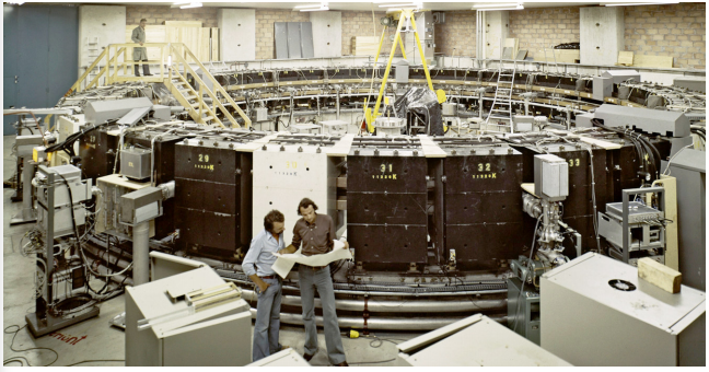
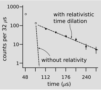
Muons were produced by an accelerator at CERN, near Geneva. A muon is essentially a heavier version of the electron. Muons undergo radioactive decay, lasting an average of only 2.197 μs before they evaporate into an electron and two neutrinos. The 1974 experiment was actually built in order to measure the magnetic properties of muons, but it produced a high-precision test of time dilation as a byproduct. Because muons have the same electric charge as electrons, they can be trapped using magnetic fields. Muons were injected into the ring shown in Figure 2.2.6, circling around it until they underwent radioactive decay. At the speed at which these muons were traveling, they had γ = 29.33, so on the average they lasted 29.33 times longer than the normal lifetime. In other words, they were like tiny alarm clocks that self-destructed at a randomly selected time. Figure 2.2.7 shows the number of radioactive decays counted, as a function of the time elapsed after a given stream of muons was injected into the storage ring. The two dashed lines show the rates of decay predicted with and without relativity. The relativistic line is the one that agrees with experiment.
11 Bailey at al., Nucl. Phys. B150(1979) 1
Example 13: Time dilation in the Pound-Rebka experiment
In the description of the Pound-Rebka experiment, the quantitative estimation of the frequency shift due to temperature was postponed. Classically, one expects only a broadening of the line, since the Doppler shift is proportional to v∥c, where v||, the component of the emitting atom’s velocity along the line of sight, averages to zero. But relativity tells us to expect that if the emitting atom is moving, its time will flow more slowly, so the frequency of the light it emits will also be systematically shifted downward. This frequency shift should increase with temperature. In other words, the Pound-Rebka experiment was designed as a test of general relativity (the equivalence principle), but this special-relativistic effect is just as strong as the relativistic one, and needed to be accounted for carefully.
In Pound and Rebka’s paper describing their experiment,12 they refer to a preliminary measurement13 in which they carefully measured this effect, showed that it was consistent with theory, and pointed out that a previous claim by Cranshaw et al. of having measured the gravitational frequency shift was vitiated by their failure to control for the temperature dependence.
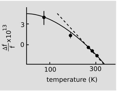
It turns out that the full Debye treatment of the lattice vibrations is not really necessary near room temperature, so we’ll simplify the thermodynamics. At absolute temperature T, the mean translational kinetic energy of each iron nucleus is (32)kT. The velocity is much less than c(= 1), so we can use the nonrelativistic expression for kinetic energy, K=(12)mv2, which gives a mean value for v2 of 3kTm. In the limit of v << 1, time dilation produces a change in frequency by a factor of 1γ, which differs from unity by approximately −v22. The relative time dilation is therefore −3kT2m, or, in metric units, −3kT2mc2. The vertical scale in figure h contains an arbitrary offset, since Pound and Rebka’s measurements were the best absolute measurements to date of the frequency. The predicted slope of −3k2mc2, however, is not arbitrary. Plugging in 57 atomic mass units for m, we find the slope to be 2.4 × 10⁻¹⁵, which, as shown in the figure is an excellent approximation (off by only 10%) near room temperature.
12 Phys. Rev. Lett. 4 (1960) 337
13 Phys. Rev. Lett. 4 (1960) 274
Geodesics and Stationary Action
One way of characterizing geodesics in spacetime is by using an action principle. This is similar to characterizing a geodesic in Euclidean space as a line of minimum length between two points. For a timelike geodesic from event P to event Q, we have a proper time τ. In Lorentz spacetime, this proper time is greater than it would have been for any non-geodesic motion from P to Q. In curved spacetime, we must weaken this statement somewhat. The proper time may not be a global maximum, but it is stationary. Stationarity means that if we vary the curve by some small amount, not moving any part of it by a coordinate distance greater than ϵ, then the change in τ is of order ϵ2.
For spacelike geodesics in Lorentz spacetime, the proper length is stationary, but small deformations of the curve can either increase or decrease the proper length. The stationary action approach does not work well for lightlike geodesics.