2.3: Affine Properties of Lorentz Geometry (Part 2)
( \newcommand{\kernel}{\mathrm{null}\,}\)
Vectors
Vectors Distinguished from Scalars
We’ve been discussing subjects like the center of mass that in freshman mechanics would be described in terms of vectors and scalars, the distinction being that vectors have a direction in space and scalars don’t. As we make the transition to relativity, we are forced to refine this distinction. For example, we used to consider time as a scalar, but the Hafele-Keating experiment shows that time is different in different frames of reference, which isn’t something that’s supposed to happen with scalars such as mass or temperature. In affine geometry, it doesn’t make much sense to say that a vector has a magnitude and direction, since non-parallel magnitudes aren’t comparable, and there is no system of angular measurement in which to describe a direction.
A better way of defining vectors and scalars is that scalars are absolute, vectors relative. If I have three apples in a bowl, then all observers in all frames of reference agree with me on the number three. But if my terrier pup pulls on the leash with a certain force vector, that vector has to be defined in relation to other things. It might be three times the strength of some force that we define as one newton, and in the same direction as the earth’s magnetic field.
In general, measurement means comparing one thing to another. The number of apples in the bowl isn’t a measurement, it’s a count.
Affine Measurement of Vectors
Before even getting into the full system of affine geometry, let’s consider the one-dimensional example of a line of time. We could use the hourly emergence of a mechanical bird from a pendulumdriven cuckoo clock to measure the rate at which the earth spins, but we could equally well take our planet’s rotation as the standard and use it to measure the frequency with which the bird pops out of the door. Once we have two things to compare against one another, measurement is reduced to counting (Figure 2.1.4). Schematically, let’s represent this measurement process with the following notation, which is part of a system called called birdtracks:3
c→e=24
Note
The system used in this book follows the one defined by Cvitanović, which was based closely on a graphical notation due to Penrose. For a more complete exposition, see the Wikipedia article “Penrose graphical notation” and Cvitanović’s online book at birdtracks.eu.
Here c represents the cuckoo clock and e the rotation of the earth. Although the measurement relationship is nearly symmetric, the arrow has a direction, because, for example, the measurement of the earth’s rotational period in terms of the clock’s frequency is c → e = (24 hr)(1 hr−1) = 24, but the clock’s period in terms of the earth’s frequency is e → c = 124. We say that the relationship is not symmetric but “dual.” By the way, it doesn’t matter how we arrange these diagrams on the page. The notations c → e and e → c mean exactly the same thing, and expressions like this can even be drawn vertically.
Suppose that e is a displacement along some one-dimensional line of time, and we want to think of it as the thing being measured. Then we expect that the measurement process represented by c produces a real-valued result and is a linear function of e. Since the relationship between c and e is dual, we expect that c also belongs to some vector space. For example, vector spaces allow multiplication by a scalar: we could double the frequency of the cuckoo clock by making the bird come out on the half hour as well as on the hour, forming 2c. Measurement should be a linear function of both vectors; we say it is “bilinear.”
Duality
The two vectors c and e have different units, hr−1 and hr, and inhabit two different one-dimensional vector spaces. The “flavor” of the vector is represented by whether the arrow goes into it or comes out. Just as we used notation like →v in freshman physics to tell vectors apart from scalars, we can employ arrows in the birdtracks notation as part of the notation for the vector, so that instead of writing the two vectors as c and e, we can notate them as c→ and →e. Performing a measurement is like plumbing. We join the two “pipes” in c→ →e and simplify to c → e.
A confusing and nonstandardized jungle of notation and terminology has grown up around these concepts. For now, let’s refer to a vector such as →e, with the arrow coming in, simply as a “vector,” and the type like c→ as a “dual vector.” In the one-dimensional example of the earth and the cuckoo clock, the roles played by the two vectors were completely equivalent, and it didn’t matter which one we expressed as a vector and which as a dual vector. Example 5 shows that it is sometimes more natural to take one quantity as a vector and another as a dual vector. Example 6 shows that we sometimes have no choice at all as to which is which.
Scaling
In birdtracks notation, a scalar is a quantity that has no external arrows at all. Since the expression c → e = 24 has no external arrows, only internal ones, it represents a scalar. This makes sense because it’s a count, and a count is a scalar.
A convenient way of summarizing all of our categories of variables is by their behavior when we convert units, i.e., when we rescale our space. If we switch our time unit from hours to minutes, the number of apples in a bowl is unchanged, the earth’s period of rotation gets 60 times bigger, and the frequency of the cuckoo clock changes by a factor of 160. In other words, a quantity u under rescaling of coordinates by a factor α becomes αpu, where the exponents −1, 0, and +1 correspond to dual vectors, scalars, and vectors, respectively. We can therefore see that these distinctions are of interest even in one dimension, contrary to what one would have expected from the freshman-physics concept of a vector as something transforming in a certain way under rotations.
Geometrical Visualization
In two dimensions, there are natural ways of visualizing the different vector spaces inhabited by vectors and dual vectors. We’ve already been describing a vector like →e as a displacement. Its vector space is the space of such displacements.4 A vector in the dual space such as c→ can be visualized as a set of parallel, evenly spaced lines on a topographic map, h2, with an arrowhead to show which way is “uphill.” The act of measurement consists of counting how many of these lines are crossed by a certain vector, h3.

Figure 2.3.8 - 1. A displacement vector. 2. A vector from the space dual to the space of displacements. 3. Measurement is reduced to counting. The cuckoo clock chimes 24 times in one rotation of the earth.
Note
In terms of the primitive notions used in the axiomatization in section 2.1, a displacement could be described as an equivalence class of segments such that for any two segments in the class AB and CD, AB and CD form a parallelogram.
Given a scalar field f, its gradient ∇f at any given point is a dual vector. In birdtracks notation, we have to indicate this by writing it with an outward-pointing arrow, (grad f)→. Because gradients occur so frequently, we have a special shorthand for them, which is simply a circle:
.png?revision=1&size=bestfit&width=58&height=41)
In the context of spacetime with a metric and curvature, we’ll see that the usual definition of the gradient in terms of partial derivatives should be modified with correction terms to form something called a covariant derivative. When we get to that point later, we’ll commandeer the circle notation for that operation.

Example 5: force is a dual vector
The dot product dW = F⋅dx for computing mechanical work becomes, in birdtracks notation,
dW=F→dx.
This shows that force is more naturally considered to be a dual vector rather than a vector. The symmetry between vectors and dual vectors is broken by considering displacements like →dx to be vectors, and this asymmetry then spreads to other quantities such as force.
The same result can be obtained from Newton’s second law; see example 21.
Example 6: Systems without a metric
The freshman-mechanics way of thinking about vectors and scalar products contains the hidden assumption that we have, besides affine measurement, an additional piece of measurement apparatus called the metric (section 3.5). Without yet having to formally define what we mean by a metric, we can say roughly that it supplies the conveniences that we’re used to having in the Euclidean plane, but that are not present in affine geometry. In particular, it allows us to define the notion that one vector is perpendicular to another vector, or that one dual vector is perpendicular to another dual vector.
Let’s start with an example where the hidden assumption is valid, and we do have a metric. Let a billiard ball of unit mass be constrained by a diagonal wall to have C ≤ 0, where C = y − x. The Lagrangian formalism just leads to the expected Newtonian expressions for the momenta conjugate to x and y, px = ˙x, py = ˙y, and these form a dual vector p→. The force of constraint is F→=dp→dt. Let w→ = (grad C)→ be the gradient of the constraint function. The vectors F→ and w→ both belong to the space of dual vectors, and they are parallel to each other. Since we do happen to have a metric in this example, it is also possible to say, as most people would, that the force is perpendicular to the wall.
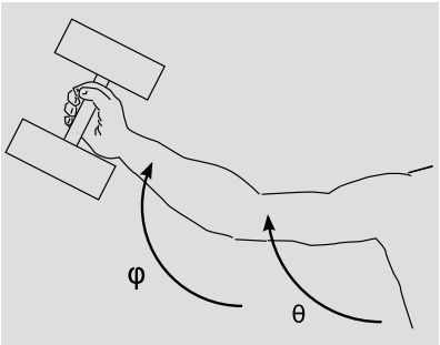
Now consider the example shown in Figure 2.1.10. The arm’s weight is negligible compared to the unit mass of the gripped weight, and both the upper and lower arm have unit length. Elbows don’t bend backward, so we have a constraint C ≤ 0, where C = θ−φ, and as before we can define define a dual vector w→ = (grad C)→ that is parallel to the line of constraint in the (θ,φ) plane. The conjugate momenta (which are actually angular momenta) turn out to be pθ=˙θ+cos(φ−θ)˙φ and a similar expression for pφ. As in the example of the billiard ball, the force of constraint is parallel to w→. There is no metric that naturally applies to the (θ,φ) plane, so we have no notion of perpendicularity, and it doesn’t make sense to say that F→ is perpendicular to the line of constraint.

Finally we remark that since four-dimensional Galilean spacetime lacks a metric (see section 3.5), the distinction between vectors and dual vectors in Galilean relativity is a real and physically important one. The only reason people were historically able to ignore this distinction was that Galilean spacetime splits into independent time and spatial parts, with the spatial part having a metric.
Example 7: No simultaneity without a metric
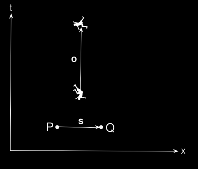
We’ll see in section 2.2 that one way of defining the distinction between Galilean and Lorentz geometry is that in Lorentzian spacetime, simultaneity is observer-dependent. Without a metric, there can be no notion of simultaneity at all, not even a frame-dependent one. In Figure 2.1.11, the fact that the observer considers events P and Q to be simultaneous is represented by the fact that the observer’s displacement vector →o is perpendicular to the displacement →s from P to Q. In affine geometry, we can’t express perpendicularity.

Abstract Index Notation
Expressions in birdtracks notation such as
.png?revision=1&size=bestfit&width=60&height=37)
can be awkward to type on a computer, which is why we’ve already been occasionally resorting to more linear notations such as (grad C)→s. As we encounter more complicated birdtracks, the diagrams will sometimes look like complicated electrical schematics, and the problem of generating them on a keyboard will get more acute. There is in fact a systematic way of representing any such expression using only ordinary subscripts and superscripts. This is called abstract index notation, and was introduced by Roger Penrose at around the same time he invented birdtracks. For practical reasons, it was the abstract index notation that caught on.
The idea is as follows. Suppose we wanted to describe a complicated birdtrack verbally, so that someone else could draw it. The diagram would be made up of various smaller parts, a typical one looking something like the scalar product u→v. The verbal instructions might be: “We have an object u with an arrow coming out of it. For reference, let’s label this arrow as a. Now remember that other object v I had you draw before? There was an arrow coming into that one, which we also labeled a. Now connect up the two arrows labeled a.”
Shortening this lengthy description to its bare minimum, Penrose renders it like this: uava. Subscripts depict arrows coming out of a symbol (think of water flowing from a tank out through a pipe below). Superscripts indicate arrows going in. When the same letter is used as both a superscript and a subscript, the two arrows are to be piped together.
Abstract index notation evolved out of an earlier one called the Einstein summation convention, in which superscripts and subscripts referred to specific coordinates. For example, we might take 0 to be the time coordinate, 1 to be x, and so on. A symbol like uγ would then indicate a component of the dual vector u, which could be its x component if γ took on the value 1. Repeated indices were summed over.
The advantage of the birdtrack and abstract index notations is that they are coordinate-independent, so that an equation written in them is valid regardless of the choice of coordinates. The Einstein and Penrose notations look very similar, so for example if we want to take a general result expressed in Penrose notation and apply it in a specific coordinate system, there is essentially no translation required. In fact, the two notations look so similar that we need an explicit way to tell which is which, so that we can tell whether or not a particular result is coordinate-independent. We therefore use the convention that Latin indices represent abstract indices, whereas Greek ones imply a specific coordinate system and can take on numerical values, e.g., γ = 1.


