4.7: Things that Aren’t Quite Tensors

This section can be skipped on a first reading.

Area, Volume, and Tensor Densities

We’ve embarked on a program of redefining every possible physical quantity as a tensor, but so far we haven’t tackled area and volume. Is there, for example, an area tensor in a locally Euclidean plane? We are encouraged to hope that there is such a thing, because in Example 3 we saw that we could cook up a measure of area with no other ingredients than the axioms of affine geometry. What kind of tensor would it be? The notions of vector and scalar from freshman mechanics are distinguished from one another by the fact that one has a direction in space and the other does not. Therefore we expect that area would be a scalar, i.e., a rank-0 tensor. But this can’t be right, for the following reason. Under a rescaling of Cartesian coordinates by a factor k, area should change by a factor of k². But by the tensor transformation laws, a rank-0 tensor is supposed to be invariant under a change of coordinates. We therefore conclude that quantities like area and volume are not tensors.

In the language of ordinary vectors and scalars in Euclidean three-space, one way to express area and volume is by using dot and cross products. The area of the parallelogram spanned by u and v is measured by the area vector u × v, and similarly the volume of the parallelepiped formed by u, v, and w can be computed as the scalar triple product u · (v × w). Both of these quantities are defined such that interchanging two of the inputs negates the output. In differential geometry, we do have a scalar product, which is defined by contracting the indices of two vectors, as in u^av_a. If we also had a a tensorial cross product, we would be able to define area and volume tensors, so we conclude that there is no tensorial cross product, i.e., an operation that would multiply two rank-1 tensors to produce a rank-1 tensor. Since one of the most important physical applications of the cross product is to calculate the angular momentum L = r × p, we find that angular momentum in relativity is either not a tensor or not a rank-1 tensor.

When someone tells you that it’s impossible to do a seemingly straightforward thing, the typical response is to look for a way to get around the supposed limitation. In the case of a locally Euclidean plane, what is to stop us from making a small, standard square, and then sliding the square around to any desired location? If we have some figure whose area we wish to measure, we can then dissect it into squares of that size and count the number of squares.

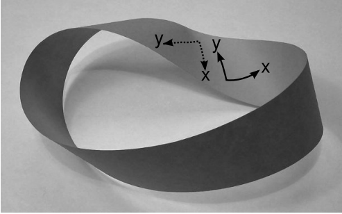
There are two problems with this plan, neither of which is completely insurmountable. First, the area vector u × v is a vector, with its orientation specified by the direction of the normal to the surface. We need this orientation, for example, when we calculate the electric flux as \(\int\) E · dA. Figure 4.6.1 shows that we cannot always define such an orientation in a consistent way. When the x − y coordinate system is slid around the Möbius strip, it ends up with the opposite orientation. In general relativity, there is not any guarantee of orientability in space — or even in time! But the vast majority of spacetimes of physical interest are in fact orientable in every desired way, and even for those that aren’t, orientability still holds in any sufficiently small neighborhood.

Figure \(\PageIndex{1}\) - A Möbius strip is not an orientable surface.

The other problem is that area has the wrong scaling properties to be a rank-0 tensor. We can get around this problem by being willing to discuss quantities that don’t transform exactly like tensors. Often we only care about transformations, such as rotations and translations, that don’t involve any scaling. We saw in section 2.2 that Lorentz boosts also have the special property of preserving area in a space-time plane containing the boost. We therefore define a tensor density as a quantity that transforms like a tensor under rotations, translations, and boosts, but that rescales and possibly flips its sign under other types of coordinate transformations. In general, the additional factor comes from the determinant d of the matrix consisting of the partial derivatives \(\frac{\partial x'^{\mu}}{\partial x^{\nu}}\) (called the Jacobian matrix). This determinant is raised to a power W, known as the weight of the tensor density. Weight zero corresponds to the case of a real tensor. The definition of the sign of W is not standardized in the literature. The convention in this book is the one used by Carroll and Weinberg, but the opposite sign is used, for example, by Misner, Thorne, and Wheeler, and in the Wikipedia article “Tensor density.”

Example 22: Area as a tensor density

In a Euclidean plane, making our rulers shorter by a factor of k causes the area measured in the new coordinates to increase by a factor of k². The rescaling is represented by a matrix of partial derivatives that is simply kI, where I is the identity matrix. The determinant is k². Therefore area is a tensor density of weight +1.

Example 23: Mass density

A piece of aluminum foil as a certain number of milligrams per square centimeter. Shrinking rulers by \(\frac{1}{k}\) causes this number to decrease by k⁻², so this mass density has W = −1.

In Weyl’s apt characterization,¹⁷ tensors represent intensities, while tensor densities measure quantity.

The Levi-Civita Symbol

Although there is no tensorial vector cross product, we can define a similar operation whose output is a tensor density. This is most easily expressed in terms of the Levi-Civita symbol \(\epsilon\). (See section 3.3 for biographical information about Levi-Civita.)

In n dimensions, the Levi-Civita symbol has n indices. It is defined so as to be totally asymmetric, in the sense that if any two of the indices are interchanged, its sign flips. This is sufficient to define the symbol completely except for an over-all scaling, which is fixed by arbitrarily taking one of the nonvanishing elements and setting it to +1. To see that this is enough to define \(\epsilon\) completely, first note that it must vanish when any index is repeated. For example, in three dimensions labeled by \(\kappa, \lambda\), and \(\mu, \epsilon_{\kappa \lambda \lambda}\) is unchanged under an interchange of the second and third indices, but it must also flip its sign under this operation, which means that it must be zero. If we arbitrarily fix \(\epsilon_{\kappa \lambda \mu} = +1\), then interchange of the second and third indices gives \(\epsilon_{\kappa \mu \lambda} = −1\), and a further interchange of the first and second yields \(\epsilon_{\mu \kappa \lambda} = +1\). Any permutation of the three distinct indices can be reached from any other by a series of such pairwise swaps, and the number of swaps is uniquely odd or even.¹⁸ In Cartesian coordinates in three dimensions, it is conventional to choose \(\epsilon_{xyz} = +1\) when x, y, and z form a right-handed spatial coordinate system. In four dimensions, we take \(\epsilon_{txyz}\) = +1 when t is future-timelike and (x, y, z) are right-handed.

In Euclidean three-space, in coordinates such that g = diag(1, 1, 1), the vector cross product A = u × v, where we have in mind the interpretation of A as area, can be expressed as \(A_{\mu} = \epsilon_{\mu \kappa \lambda} u^{\kappa} v^{\lambda}\).

Note

For a proof, see the Wikipedia article “Parity of a permutation.”

Exercise \(\PageIndex{1}\)

Self-check: Check that this matches up with the more familiar definition of the vector cross product.

Now suppose that we want to generalize to curved spaces, where g cannot be constant. There are two ways to proceed.

Tensorial \(\epsilon\)

One is to let \(\epsilon\) have the values 0 and ±1 at some arbitrarily chosen point, in some arbitrarily chosen coordinate system, but to let it transform like a tensor. Then \(A_{\mu} = \epsilon_{\mu \kappa \lambda} u^{\kappa} v^{\lambda}\) needs to be modified, since the right-hand side is a tensor, and that would make A a tensor, but if A is an area we don’t want it to transform like a 1-tensor. We therefore need to revise the definition of area to be \(A_{\mu} = g^{−1/2} \epsilon_{\mu \kappa \lambda} u^{\kappa} v^{\lambda}\), where g is the determinant of the lower-index form of the metric. The following two examples justify this procedure in a locally Euclidean three-space.

Example 24: Scaling coordinates with tensorial \(\epsilon\)

Then scaling of coordinates by k scales all the elements of the metric by k⁻², g by k⁻⁶, g^−1/2 by k³, \(\epsilon_{\mu \kappa \lambda}\) by k⁻³, and \(u^{\kappa} v^{\lambda}\) by k². The result is to scale A_\(\mu\) by k⁺³⁻³⁺² = k², which makes sense if A is an area.

Example 25: oblique coordinates with tensorial \(\epsilon\)

In oblique coordinates (example 9), the two basis vectors have unit length but are at an angle \(\phi \neq \frac{\pi}{2}\) to one another. The determinant of the metric is g = sin² \(\phi\), so \(\sqrt{g} = \sin \phi\), which is exactly the correction factor needed in order to get the right area when u and v are the two basis vectors.

This procedure works more generally, the sole modification being that in a space such as a locally Lorentzian one where g < 0 we need to use \(\sqrt{−g}\) as the correction factor rather than \(\sqrt{g}\).

Tensor-density \(\epsilon\)

The other option is to let \(\epsilon\) have the same 0 and ±1 values at all points. Then is clearly not a tensor, because it doesn’t scale by a factor of kⁿ when the coordinates are scaled by k; \(\epsilon\) is a tensor density with weight −1 for the upper-index version and +1 for the lower-index one. The relation \(A_{\mu} = \epsilon_{\mu \kappa \lambda} u^{\kappa} v^{\lambda}\) gives an area that is a tensor density, not a tensor, because A is not written in terms of purely tensorial quantities. Scaling the coordinates by k leaves \(\epsilon_{\mu \kappa \lambda}\) unchanged, scales up \(u^{\kappa} v^{\lambda}\) by k², and scales up the area by k², as expected.

Unfortunately, there is no consistency in the literature as to whether \(\epsilon\) should be a tensor or a tensor density. Some authors define both a tensor and a nontensor version, with notations like \(\epsilon\) and \(\tilde{\epsilon}\), or¹⁹ \(\epsilon_{0123}\) and [0123]. Others avoid writing the letter \(\epsilon\) completely.²⁰ The tensor-density version is convenient because we always know that its value is 0 or ±1. The tensor version has the advantage that it transforms as a tensor.

Spacetime Volume

We saw in section 2.2 that area in the 1 + 1-dimensional plane of flat spacetime is preserved by a Lorentz boost. This makes sense because when we express the area spanned by a parallelogram with edges p and q as \(\epsilon^{ab} p_{a} s_{b}\), all the indices have been contracted, leaving a rank-0 tensor density. In 3 + 1 dimensions, we have the spacetime volume V = \(\epsilon^{abcd} p_{a} q_{b} r_{c} s_{d}\) spanned by the paralellepiped with edges p, q, r, and s. A typical situation in which this volume is nonzero would be that in which one of the vectors is timelike and the other three spacelike. Let the timelike one be p. Assume |p| = 1, since an example with |p| ≠ 1 can be reduced to this by scaling. Then p can be interpreted as the velocity vector of some observer, and V as the spatial volume that the observer says is spanned by the 3-paralellepiped with edges q, r, and s.

Angular Momentum

As discussed above, angular momentum cannot be a rank-1 tensor. One approach is to define a rank-2 angular momentum tensor L^ab = r^ap^b − r^bp^a.

In a frame whose origin is instantaneously moving along with a certain system’s center of mass at a certain time, the time-space components of L vanish, and the components L^yz, L^zx, and L^xy coincide in the nonrelativistic limit with the x, y, and z components of the Newtonian angular momentum vector. We can also define a three-dimensional object \(L^{a} = \epsilon_{abc} L^{bc}\) (with three-dimensional tensor-density \(\epsilon\) in the spatial dimensions) that doesn’t transform like a tensor.

References

¹⁷ Hermann Weyl, “Space-Time-Matter,” 1922, p. 109, available online at archive.org/details/spacetimematter00weyluoft.

¹⁹ Misner, Thorne, and Wheeler

²⁰ Hawking and Ellis