
3.6: The Metric (Part 1)
- Page ID
- 11284

\( \newcommand{\vecs}[1]{\overset { \scriptstyle \rightharpoonup} {\mathbf{#1}} } \)
\( \newcommand{\vecd}[1]{\overset{-\!-\!\rightharpoonup}{\vphantom{a}\smash {#1}}} \)
\( \newcommand{\dsum}{\displaystyle\sum\limits} \)
\( \newcommand{\dint}{\displaystyle\int\limits} \)
\( \newcommand{\dlim}{\displaystyle\lim\limits} \)
\( \newcommand{\id}{\mathrm{id}}\) \( \newcommand{\Span}{\mathrm{span}}\)
( \newcommand{\kernel}{\mathrm{null}\,}\) \( \newcommand{\range}{\mathrm{range}\,}\)
\( \newcommand{\RealPart}{\mathrm{Re}}\) \( \newcommand{\ImaginaryPart}{\mathrm{Im}}\)
\( \newcommand{\Argument}{\mathrm{Arg}}\) \( \newcommand{\norm}[1]{\| #1 \|}\)
\( \newcommand{\inner}[2]{\langle #1, #2 \rangle}\)
\( \newcommand{\Span}{\mathrm{span}}\)
\( \newcommand{\id}{\mathrm{id}}\)
\( \newcommand{\Span}{\mathrm{span}}\)
\( \newcommand{\kernel}{\mathrm{null}\,}\)
\( \newcommand{\range}{\mathrm{range}\,}\)
\( \newcommand{\RealPart}{\mathrm{Re}}\)
\( \newcommand{\ImaginaryPart}{\mathrm{Im}}\)
\( \newcommand{\Argument}{\mathrm{Arg}}\)
\( \newcommand{\norm}[1]{\| #1 \|}\)
\( \newcommand{\inner}[2]{\langle #1, #2 \rangle}\)
\( \newcommand{\Span}{\mathrm{span}}\) \( \newcommand{\AA}{\unicode[.8,0]{x212B}}\)
\( \newcommand{\vectorA}[1]{\vec{#1}} % arrow\)
\( \newcommand{\vectorAt}[1]{\vec{\text{#1}}} % arrow\)
\( \newcommand{\vectorB}[1]{\overset { \scriptstyle \rightharpoonup} {\mathbf{#1}} } \)
\( \newcommand{\vectorC}[1]{\textbf{#1}} \)
\( \newcommand{\vectorD}[1]{\overrightarrow{#1}} \)
\( \newcommand{\vectorDt}[1]{\overrightarrow{\text{#1}}} \)
\( \newcommand{\vectE}[1]{\overset{-\!-\!\rightharpoonup}{\vphantom{a}\smash{\mathbf {#1}}}} \)
\( \newcommand{\vecs}[1]{\overset { \scriptstyle \rightharpoonup} {\mathbf{#1}} } \)
\(\newcommand{\longvect}{\overrightarrow}\)
\( \newcommand{\vecd}[1]{\overset{-\!-\!\rightharpoonup}{\vphantom{a}\smash {#1}}} \)
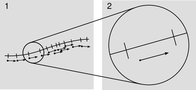
\(\newcommand{\avec}{\mathbf a}\) \(\newcommand{\bvec}{\mathbf b}\) \(\newcommand{\cvec}{\mathbf c}\) \(\newcommand{\dvec}{\mathbf d}\) \(\newcommand{\dtil}{\widetilde{\mathbf d}}\) \(\newcommand{\evec}{\mathbf e}\) \(\newcommand{\fvec}{\mathbf f}\) \(\newcommand{\nvec}{\mathbf n}\) \(\newcommand{\pvec}{\mathbf p}\) \(\newcommand{\qvec}{\mathbf q}\) \(\newcommand{\svec}{\mathbf s}\) \(\newcommand{\tvec}{\mathbf t}\) \(\newcommand{\uvec}{\mathbf u}\) \(\newcommand{\vvec}{\mathbf v}\) \(\newcommand{\wvec}{\mathbf w}\) \(\newcommand{\xvec}{\mathbf x}\) \(\newcommand{\yvec}{\mathbf y}\) \(\newcommand{\zvec}{\mathbf z}\) \(\newcommand{\rvec}{\mathbf r}\) \(\newcommand{\mvec}{\mathbf m}\) \(\newcommand{\zerovec}{\mathbf 0}\) \(\newcommand{\onevec}{\mathbf 1}\) \(\newcommand{\real}{\mathbb R}\) \(\newcommand{\twovec}[2]{\left[\begin{array}{r}#1 \\ #2 \end{array}\right]}\) \(\newcommand{\ctwovec}[2]{\left[\begin{array}{c}#1 \\ #2 \end{array}\right]}\) \(\newcommand{\threevec}[3]{\left[\begin{array}{r}#1 \\ #2 \\ #3 \end{array}\right]}\) \(\newcommand{\cthreevec}[3]{\left[\begin{array}{c}#1 \\ #2 \\ #3 \end{array}\right]}\) \(\newcommand{\fourvec}[4]{\left[\begin{array}{r}#1 \\ #2 \\ #3 \\ #4 \end{array}\right]}\) \(\newcommand{\cfourvec}[4]{\left[\begin{array}{c}#1 \\ #2 \\ #3 \\ #4 \end{array}\right]}\) \(\newcommand{\fivevec}[5]{\left[\begin{array}{r}#1 \\ #2 \\ #3 \\ #4 \\ #5 \\ \end{array}\right]}\) \(\newcommand{\cfivevec}[5]{\left[\begin{array}{c}#1 \\ #2 \\ #3 \\ #4 \\ #5 \\ \end{array}\right]}\) \(\newcommand{\mattwo}[4]{\left[\begin{array}{rr}#1 \amp #2 \\ #3 \amp #4 \\ \end{array}\right]}\) \(\newcommand{\laspan}[1]{\text{Span}\{#1\}}\) \(\newcommand{\bcal}{\cal B}\) \(\newcommand{\ccal}{\cal C}\) \(\newcommand{\scal}{\cal S}\) \(\newcommand{\wcal}{\cal W}\) \(\newcommand{\ecal}{\cal E}\) \(\newcommand{\coords}[2]{\left\{#1\right\}_{#2}}\) \(\newcommand{\gray}[1]{\color{gray}{#1}}\) \(\newcommand{\lgray}[1]{\color{lightgray}{#1}}\) \(\newcommand{\rank}{\operatorname{rank}}\) \(\newcommand{\row}{\text{Row}}\) \(\newcommand{\col}{\text{Col}}\) \(\renewcommand{\row}{\text{Row}}\) \(\newcommand{\nul}{\text{Nul}}\) \(\newcommand{\var}{\text{Var}}\) \(\newcommand{\corr}{\text{corr}}\) \(\newcommand{\len}[1]{\left|#1\right|}\) \(\newcommand{\bbar}{\overline{\bvec}}\) \(\newcommand{\bhat}{\widehat{\bvec}}\) \(\newcommand{\bperp}{\bvec^\perp}\) \(\newcommand{\xhat}{\widehat{\xvec}}\) \(\newcommand{\vhat}{\widehat{\vvec}}\) \(\newcommand{\uhat}{\widehat{\uvec}}\) \(\newcommand{\what}{\widehat{\wvec}}\) \(\newcommand{\Sighat}{\widehat{\Sigma}}\) \(\newcommand{\lt}{<}\) \(\newcommand{\gt}{>}\) \(\newcommand{\amp}{&}\) \(\definecolor{fillinmathshade}{gray}{0.9}\)Consider a coordinate x defined along a certain curve, which is not necessarily a geodesic. For concreteness, imagine this curve to exist in two spacelike dimensions, which we can visualize as the surface of a sphere embedded in Euclidean 3-space. These concrete features are not strictly necessary, but they drive home the point that we should not expect to be able to define x so that it varies at a steady rate with elapsed distance; for example, we know that it will not be possible to define a two-dimensional Cartesian grid on the surface of a sphere. In the figure, the tick marks are therefore not evenly spaced. This is perfectly all right, given the coordinate invariance of general relativity. Since the incremental changes in x are equal, I’ve represented them below the curve as little vectors of equal length. They are the wrong length to represent distances along the curve, but this wrongness is an inevitable fact of life in relativity.

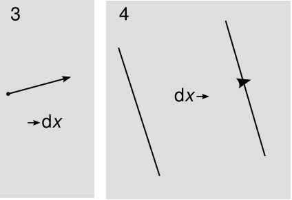
Now suppose we want to integrate the arc length of a segment of this curve. The little vectors are infinitesimal. In the integrated length, each little vector should contribute some amount, which is a scalar. This scalar is not simply the magnitude of the vector, \(ds \neq \sqrt{d \textbf{x} \cdot d \textbf{x}}\), since the vectors are the wrong length. Figure \(\PageIndex{1}\) is clearly reminiscent of the geometrical picture of vectors and dual vectors developed earlier. But the purely affine notion of vectors and their duals is not enough to define the length of a vector in general; it is only sufficient to define a length relative to other lengths along the same geodesic. When vectors lie along different geodesics, we need to be able to specify the additional conversion factor that allows us to compare one to the other. The piece of machinery that allows us to do this is called a metric.
Fixing a metric allows us to define the proper scaling of the tick marks relative to the arrows at a given point, i.e., in the birdtracks notation it gives us a natural way of taking a displacement vector such as →s, with the arrow pointing into the symbol, and making a corresponding dual vector s→, with the arrow coming out. This is a little like cloning a person but making the clone be of the opposite sex. Hooking them up like s→s then tells us the squared magnitude of the vector. For example, if →dx is an infinitesimal timelike displacement, then dx→dx is the squared time interval dx2 measured by a clock traveling along that displacement in spacetime. (Note that in the notation dx2, it’s clear that dx is a scalar, because unlike →dx and dx→ it doesn’t have any arrow coming in or out of it.) Figure \(\PageIndex{2}\) shows the resulting picture.
In the abstract index notation introduced earlier, the vectors →dx and dx→ are written dxa and dxa. When a specific coordinate system has been fixed, we write these with concrete, Greek indices, \(dx^\mu\) and \(dx_{\mu}\). In an older and conceptually incompatible notation and terminology due to Sylvester (1853), one refers to \(dx_{\mu}\) as a contravariant vector, and \(dx^\mu\) as covariant. The confusing terminology is summarized in Appendix C.
The assumption that a metric exists is nontrivial. There is no metric in Galilean spacetime, for example, since in the limit c → \(\infty\) the units used to measure timelike and spacelike displacements are not comparable. Assuming the existence of a metric is equivalent to assuming that the universe holds at least one physically manipulable clock or ruler that can be moved over long distances and accelerated as desired. In the distant future, large and causally isolated regions of the cosmos may contain only massless particles such as photons, which cannot be used to build clocks (or, equivalently, rulers); the physics of these regions will be fully describable without a metric. If, on the other hand, our world contains not just zero or one but two or more clocks, then the metric hypothesis requires that these clocks maintain a consistent relative rate when accelerated along the same world-line. This consistency is what allows us to think of relativity as a theory of space and time rather than a theory of clocks and rulers. There are other relativistic theories of gravity besides general relativity, and some of these violate this hypothesis.
Given a dx\(\mu\), how do we find its dual dx\(\mu\), and vice versa? In one dimension, we simply need to introduce a real number g as a correction factor. If one of the vectors is shorter than it should be in a certain region, the correction factor serves to compensate by making its dual proportionately longer. The two possible mappings (covariant to contravariant and contravariant to covariant) are accomplished with factors of g and 1/g. The number g is the metric, and it encodes all the information about distances. For example, if \(\phi\) represents longitude measured at the arctic circle, then the metric is the only source for the datum that a displacement d\(\phi\) corresponds to 2540 km per radian.
Now let’s generalize to more than one dimension. Because globally Cartesian coordinate systems can’t be imposed on a curved space, the constant-coordinate lines will in general be neither evenly spaced nor perpendicular to one another. If we construct a local set of basis vectors lying along the intersections of the constant coordinate surfaces, they will not form an orthonormal set. We would like to have an expression of the form
\[ds^{2} = \sum dx^{\mu} dx_{\mu}\]
for the squared arc length, and using the Einstein summation notation this becomes
\[ds^{2} = dx^{\mu} dx_{\mu}\]
The Euclidean Metric
For Cartesian coordinates in a Euclidean plane, where one doesn’t normally bother with the distinction between covariant and contravariant vectors, this expression for \(ds^2\) is simply the Pythagorean theorem, summed over two values of \(\mu\) for the two coordinates:
\[ds^{2} = dx^{\mu} dx_{\mu} = dx^{2} + dy^{2}\]
The symbols dx, ds0, dx0, and dx0 are all synonyms, and likewise for dy, ds1, dx1, and dx1. (Because notations such as ds1 force the reader to keep track of which digits have been assigned to which letters, it is better practice to use notation such as dy or dsy; the latter notation could in principle be confused with one in which y was a variable taking on values such as 0 or 1, but in reality we understand it from context, just as we understand that the d’s in \(\frac{dy}{dx}\) are not referring to some variable d that stands for a number.)
In the non-Euclidean case, the Pythagorean theorem is false; \(dx^\mu\) and \(dx_\mu\) are no longer synonyms, so their product is no longer simply the square of a distance. To see this more explicitly, let’s write the expression so that only the covariant quantities occur. By local flatness, the relationship between the covariant and contravariant vectors is linear, and the most general relationship of this kind is given by making the metric a symmetric matrix \(g_{\mu \nu}\). Substituting \(dx_{\mu} = g_{\mu \nu} x^{\nu}\), we have
\[ds^{2} = g_{\mu \nu} dx^{\mu} dx^{\nu}\]
where there are now implied sums over both µ and ν. Notice how implied sums occur only when the repeated index occurs once as a superscript and once as a subscript; other combinations are ungrammatical.
Exercise \(\PageIndex{1}\)
Self-check: Why does it make sense to demand that the metric be symmetric?
Earlier we encountered the distinction among scalars, vectors, and dual vectors. These are specific examples of tensors, which can be expressed in the birdtracks notation as objects with m arrows coming in and n coming out, or. In index notation, we have m superscripts and n subscripts. A scalar has m = n = 0. A dual vector has (m, n) = (0, 1), a vector (1, 0), and the metric (0, 2). We refer to the number of indices as the rank of the tensor. Tensors are discussed in more detail, and defined more rigorously, in chapter 4. For our present purposes, it is important to note that just because we write a symbol with subscripts or superscripts, that doesn’t mean it deserves to be called a tensor. This point can be understood in the more elementary context of Newtonian scalars and vectors. For example, we can define a Euclidean “vector” u = (m, T, e), where m is the mass of the moon, T is the temperature in Chicago, and e is the charge of the electron. This creature u doesn’t deserve to be called a vector, because it doesn’t behave as a vector under rotation. The general philosophy is that a tensor is something that has certain properties under changes of coordinates. For example, we’ve already seen earlier the different scaling behavior of tensors with ranks (1, 0), (0, 0), and (0, 1).
When discussing the symmetry of rank-2 tensors, it is convenient to introduce the following notation:
\[T_{(ab)} = \frac{1}{2} (T_{ab} + T_{ba})\]
\[T_{[ab]} = \frac{1}{2} (T_{ab} - T_{ba})\]
Any Tab can be split into symmetric and antisymmetric parts. This is similar to writing an arbitrary function as a sum of and odd function and an even function. The metric has only a symmetric part: g(ab) = gab, and g[ab] = 0. This notation is generalized to ranks greater than 2 later.
Exercise \(\PageIndex{2}\)
Self-check: Characterize an antisymmetric rank-2 tensor in two dimensions.
Example 7: A change of scale
- Suppose we start by describing the Euclidean plane with a certain set of Cartesian coordinates, but then want to change to a new set of coordinates that are rescaled compared to the original ones. How is the effect of this rescaling represented in g?.
- If we change our units of measurement so that \(x_{\mu} \rightarrow \alpha x^{\mu}\), while demanding that ds2 come out the same, then we need \(g_{\mu \nu} \rightarrow \alpha^{−2} g_{\mu \nu}\).
Comparing with section 2.1, we deduce the general rule that a tensor of rank (m, n) transforms under scaling by picking up a factor of \(\alpha^{m−n}\).
This whole notion of scaling and units in general relativity turns out to be nontrivial and interesting. See section 5.11, for a more detailed discussion.
Example 8: polar coordinates
Consider polar coordinates (r, \(\theta\)) in a Euclidean plane. The constant-coordinate curves happen to be orthogonal everywhere, so the off-diagonal elements of the metric gr\(\theta\) and g\(\theta\)r vanish. Infinitesimal coordinate changes dr and d\(\theta\) correspond to infinitesimal displacements dr and r d\(\theta\) in orthogonal directions, so by the Pythagorean theorem, ds2 = dr2 + r2 d\(\theta\)2, and we read off the elements of the metric grr = 1 and g\(\theta\)\(\theta\) = r2.
Notice how in example 8 we started from the generally valid relation \(ds^{2} = g_{\mu \nu} dx^{\mu} dx^{\nu}\), but soon began writing down facts like g\(\theta\)\(\theta\) = r2 that were only valid in this particular coordinate system. To make it clear when this is happening, we maintain the distinction between abstract Latin indices and concrete Greek indices introduced earlier. For example, we can write the general expression for squared differential arc length with Latin indices,
\[ds^{2} = g_{ij} dx^{i} dx^{j},\]
because it holds regardless of the coordinate system, whereas the vanishing of the off-diagonal elements of the metric in Euclidean polar coordinates has to be written as g\(\mu \nu\) = 0 for \(\mu \neq \nu\), since it would in general be false if we used a different coordinate system to describe the same Euclidean plane.
Example 9: Oblique Cartesian coordinates
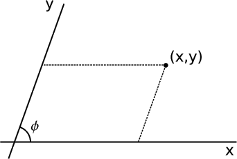
- Oblique Cartesian coordinates are like normal Cartesian coordinates in the plane, but their axes are at at an angle \(\phi \neq \frac{\pi}{2}\) to one another. Find the metric in these coordinates. The space is globally Euclidean.
- Since the coordinates differ from Cartesian coordinates only in the angle between the axes, not in their scales, a displacement dxi along either axis, i = 1 or 2, must give ds = dx, so for the diagonal elements we have g11 = g22 = 1. The metric is always symmetric, so g12 = g21. To fix these off-diagonal elements, consider a displacement by ds in the direction perpendicular to axis 1. This changes the coordinates by dx1 = − ds cot \(\phi\) and dx2 = ds cos \(\phi\). We then have
\[\begin{split} ds^{2} &= g_{ij} dx^{i} dx^{j} \\ &= ds^{2} (\cot^{2} \phi + csc^{2} \phi - 2g_{12} \cot \phi \csc \phi) \\ g_{12} &= \cos \phi \ldotp \end{split}\]
Example 10: area
In one dimension, g is a single number, and lengths are given by ds = \(\sqrt{g}\) dx. The square root can also be understood through example 7, in which we saw that a uniform rescaling x → \(\alpha\)x is reflected in \(g_{\mu \nu} \rightarrow \alpha^{−2} g_{\mu \nu}\).
In two-dimensional Cartesian coordinates, multiplication of the width and height of a rectangle gives the element of area \(dA = \sqrt{g_{11} g_{22}} dx^{1} dx^{2}\). Because the coordinates are orthogonal, g is diagonal, and the factor of \(\sqrt{g_{11} g_{22}}\) is identified as the square root of its determinant, so dA = \(\sqrt{|g|}\) dx1 dx2. Note that the scales on the two axes are not necessarily the same, g11 ≠ g22.
The same expression for the element of area holds even if the coordinates are not orthogonal. In example 9, for instance, we have \(\sqrt{|g|} = \sqrt{1 − \cos^{2} \phi} = \sin \phi\), which is the right correction factor corresponding to the fact that dx1 and dx2 form a parallelepiped rather than a rectangle.
Example 11: area of a sphere
For coordinates \((\theta, \phi)\) on the surface of a sphere of radius r, we have, by an argument similar to that of example 8 \(g_{\theta \theta} = r^{2}, g_{\phi \phi} = r^{2} \sin^{2} \theta, g_{\theta \phi} = 0\). The area of the sphere is
\[\begin{split} A &= \int dA \\ &= \int \int \sqrt{|g|} d \theta d \phi \\ &= r^{2} \int \int \sin \theta d \theta d \phi \\ &= 4 \pi r^{2} \end{split}\]
Example 12: inverse of the metric
- Relate gij to gij.
- The notation is intended to treat covariant and contravariant vectors completely symmetrically. The metric with lower indices gij can be interpreted as a change-of-basis transformation from a contravariant basis to a covariant one, and if the symmetry of the notation is to be maintained, gij must be the corresponding inverse matrix, which changes from the covariant basis to the contravariant one. The metric must always be invertible.
In the one-dimensional case, the metric at any given point was simply some number g, and we used factors of g and 1/g to convert back and forth between covariant and contravariant vectors. Example 12 makes it clear how to generalize this to more dimensions:
\[\begin{split} x_{a} &= g_{ab} x^{b} \\ x^{a} &= g^{ab} x_{b} \end{split}\]
This is referred to as raising and lowering indices. There is no need to memorize the positions of the indices in these rules; they are the only ones possible based on the grammatical rules, which are that summation only occurs over top-bottom pairs, and upper and lower indices have to match on both sides of the equals sign. This whole system, introduced by Einstein, is called “index-gymnastics” notation.
Example 13: Raising and lowering indices on a rank-two tensor
In physics we encounter various examples of matrices, such as the moment of inertia tensor from classical mechanics. These have two indices, not just one like a vector. Again, the rules for raising and lowering indices follow directly from grammar. For example,
\[A^{a}_{b} = g^{ac} A_{cb}\]
and
\[A_{ab} = g_{ac} g_{bd} A^{cd} \ldotp\]
Example 14: A matrix operating on a vector
The row and column vectors from linear algebra are the covariant and contravariant vectors in our present terminology. (The convention is that covariant vectors are row vectors and contravariant ones column vectors, but I don’t find this worth memorizing.) What about matrices? A matrix acting on a column vector gives another column vector, q = Up Translating this into indexgymnastics notation, we have
\[q^{a} = U^{\ldots} \ldots p^{b},\]
where we want to figure out the correct placement of the indices on U. Grammatically, the only possible placement is
\[q^{a} = U^{a}_{b} p^{b} \ldotp\]
This shows that the natural way to represent a column-vector-to-column-vector linear operator is as a rank-2 tensor with one upper index and one lower index.
In birdtracks notation, a rank-2 tensor is something that has two arrows connected to it. Our example becomes → q =→ U → p. That the result is itself an upper-index vector is shown by the fact that the right-hand-side taken as a whole has a single external arrow coming into it.
The distinction between vectors and their duals may seem irrelevant if we can always raise and lower indices at will. We can’t always do that, however, because in many perfectly ordinary situations there is no metric. See example 6.
The Lorentz Music
In a locally Euclidean space, the Pythagorean theorem allows us to express the metric in local Cartesian coordinates in the simple form
\[g_\mu\mu = +1, g\mu\nu = 0\]
i.e.,
\[g = diag(+1, +1, . . . , +1).\]
This is not the appropriate metric for a locally Lorentz space. The axioms of Euclidean geometry E3 (existence of circles) and E4 (equality of right angles) describe the theory’s invariance under rotations, and the Pythagorean theorem is consistent with this, because it gives the same answer for the length of a vector even if its components are reexpressed in a new basis that is rotated with respect to the original one. In a Lorentzian geometry, however, we care about invariance under Lorentz boosts, which do not preserve the quantity \(t^2 + x^2\). It is not circles in the (t, x) plane that are invariant, but light cones, and this is described by giving gtt and gxx opposite signs and equal absolute values. A lightlike vector (t, x), with t = x, therefore has a magnitude of exactly zero
\[s^{2} = g_{tt} t^{2} + g_{xx} x^{2} = 0,\]
and this remains true after the Lorentz boost (t, x) → (\(\gamma\)t, \(\gamma\)x). It is a matter of convention which element of the metric to make positive and which to make negative. In this book, I’ll use gtt = +1 and gxx = −1, so that g = diag(+1, −1). This has the advantage that any line segment representing the timelike world-line of a physical object has a positive squared magnitude; the forward flow of time is represented as a positive number, in keeping with the philosophy that relativity is basically a theory of how causal relationships work. With this sign convention, spacelike vectors have positive squared magnitudes, timelike ones negative. The same convention is followed, for example, by Penrose. The opposite version, with g = diag(−1, +1) is used by authors such as Wald and Misner, Thorne, and Wheeler.
Our universe does not have just one spatial dimension, it has three, so the full metric in a Lorentz frame is given by
\[g = diag(+1, −1, −1, −1).\]
Example 15: Mixed covariant-contravariant form of the metric
In example 13, we saw how to raise and lower indices on a rank-two tensor, and example 14 showed that it is sometimes natural to consider the form in which one index is raised and one lowered. The metric itself is a rank-two tensor, so let’s see what happens when we compute the mixed form gab from the lower-index form. In general, we have
\[A^{a}_{b} = g^{ac} A_{cb},\]
and substituting g for A gives
\[g_{b}^{a} = g^{ac} g_{cb} \ldotp\]
But we already know that g... is simply the inverse matrix of g... (example 12), which means that gab is simply the identity matrix. That is, whereas a quantity like gab or gab carries all the information about our system of measurement at a given point, gab carries no information at all. Where gab or gab can have both positive and negative elements, elements that have units, and off-diagonal elements, gab is just a generic symbol carrying no information other than the dimensionality of the space.
The metric tensor is so commonly used that it is simply left out of birdtrack diagrams. Consistency is maintained because because gab is the identity matrix, so → g → is the same as →→.