4.6: Conservation Laws

No General Conservation Laws

Some of the first tensors we discussed were mass and charge, both rank-0 tensors, and the rank-1 momentum tensor, which contains both the classical energy and the classical momentum. Physicists originally decided that mass, charge, energy, and momentum were interesting because these things were found to be conserved. This makes it natural to ask how conservation laws can be formulated in relativity. We’re used to stating conservation laws casually in terms of the amount of something in the whole universe, e.g., that classically the total amount of mass in the universe stays constant. Relativity does allow us to make physical models of the universe as a whole, so it seems as though we ought to be able to talk about conservation laws in relativity.

We can’t.

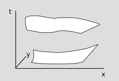
First, how do we define “stays constant?” Simultaneity isn’t well-defined, so we can’t just take two snapshots, call them initial and final, and compare the total amount of, say, electric charge in each snapshot. This difficulty isn’t insurmountable. As in figure a, we can arbitrarily pick out three-dimensional spacelike surfaces — one initial and one final — and integrate the charge over each one. A law of conservation of charge would say that no matter what spacelike surface we picked, the total charge on each would be the same.

Figure \(\PageIndex{1}\) - Two spacelike surfaces.

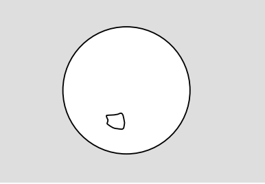
Next there’s the issue that the integral might diverge, especially if the universe was spatially infinite. For now, let’s assume a spatially finite universe. For simplicity, let’s assume that it has the topology of a three-sphere (see section 8.2 for reassurance that this isn’t physically unreasonable), and we can visualize it as a two-sphere.

Figure \(\PageIndex{2}\) - We define a boundary around a region whose charge we want to measure.

In the case of the momentum four-vector, what coordinate system would we express it in? In general, we do not even expect to be able to define a smooth, well-behaved coordinate system that covers the entire universe, and even if we did, it would not make sense to add a vector expressed in that coordinate system at point A to another vector from point B; the best we could do would be to parallel-transport the vectors to one point and then add them, but parallel transport is path-dependent. (Similar issues occur with angular momentum.) For this reason, let’s restrict ourselves to the easier case of a scalar, such as electric charge.

Figure \(\PageIndex{3}\) - This boundary cuts the sphere into equal parts.

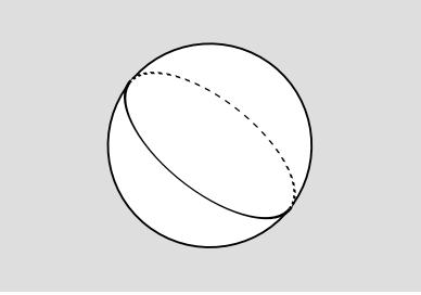
But now we’re in real trouble. How would we go about actually measuring the total electric charge of the universe? The only way to do it is to measure electric fields, and then apply Gauss’s law. This requires us to single out some surface that we can integrate the flux over, as in Figure 4.5.2. This would really be a two-dimensional surface on the three-sphere, but we can visualize it as a one-dimensional surface — a closed curve — on the two-sphere. But now suppose this curve is a great circle, Figure 4.5.3. If we measure a nonvanishing total flux across it, how do we know where the charge is? It could be on either side.

The conclusion is that conservation laws only make sense in relativity under very special circumstances.¹⁶ We do not have anything like over-arching, global principles of conservation. As an example of the appropriate special circumstances, section 6.2 shows how to define conserved quantities, which behave like energy and momentum, for the motion of a test particle in a particular metric that has a certain symmetry. This is generalized in section 7.1 to a general, global conservation law corresponding to every continuous symmetry of a spacetime.

Note

For another argument leading to the same conclusion, see section 7.5.

Conservation of Angular Momentum and Frame Dragging

Another special case where conservation laws work is that if the spacetime we’re studying gets very flat at large distances from a small system we’re studying, then we can define a far-away boundary that surrounds the system, measure the flux through that boundary, and find the system’s charge. For such asymptotic flatness spacetimes, we can also get around the problems that crop up with conserved vectors, such as momentum. (Asymptotic flatness is discussed in more detail in section 7.4.) If the spacetime far away is nearly flat, then parallel transport loses its path-dependence, so we can unambiguously define a notion of parallel-transporting all the contributions to the flux to one arbitrarily chosen point P and then adding them. Asymptotic flatness also allows us to define an approximate notion of a global Lorentz frame, so that the choice of P doesn’t matter.

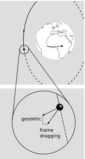
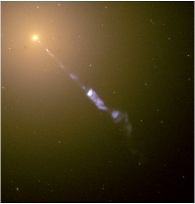
As an example, Figure 4.5.4 shows a jet of matter being ejected from the galaxy M87 at ultrarelativistic fields. The blue color of the jet in the visible-light image comes from synchrotron radiation, which is the electromagnetic radiation emitted by relativistic charged particles accelerated by a magnetic field. The jet is believed to be coming from a supermassive black hole at the center of M87. The emission of the jet in a particular direction suggests that the black hole is not spherically symmetric. It seems to have a particular axis associated with it. How can this be? Our sun’s spherical symmetry is broken by the existence of externally observable features such as sunspots and the equatorial bulge, but the only information we can get about a black hole comes from its external gravitational (and possibly electromagnetic) fields. It appears that something about the spacetime metric surrounding this black hole breaks spherical symmetry, but preserves symmetry about some preferred axis. What aspect of the initial conditions in the formation of the hole could have determined such an axis? The most likely candidate is the angular momentum. We are thus led to suspect that black holes can possess angular momentum, that angular momentum preserves information about their formation, and that angular momentum is externally detectable via its effect on the spacetime metric.

Figure \(\PageIndex{4}\) - A relativistic jet.

What would the form of such a metric be? Spherical coordinates in flat spacetime give a metric like this:

\[ds^{2} = dt^{2} - dr^{2} - r^{2} d \theta^{2} - r^{2} \sin^{2} \theta d \phi^{2} \ldotp\]

We’ll see in chapter 6 that for a non-rotating black hole, the metric is of the form

\[ds^{2} = (\ldots) dt^{2} - (\ldots) dr^{2} - r^{2} d \theta^{2} - r^{2} \sin^{2} \theta d \phi^{2},\]

where (. . .) represents functions of r. In fact, there is nothing special about the metric of a black hole, at least far away; the same external metric applies to any spherically symmetric, non-rotating body, such as the moon. Now what about the metric of a rotating body? We expect it to have the following properties:

1. It has terms that are odd under time-reversal, corresponding to reversal of the body’s angular momentum.
2. Similarly, it has terms that are odd under reversal of the differential d\(\phi\) of the azimuthal coordinate.
3. The metric should have axial symmetry, i.e., it should be independent of \(\phi\).

Restricting our attention to the equatorial plane \(\theta = \frac{\pi}{2}\), the simplest modification that has these three properties is to add a term of the form

\[f(\ldots) L d \phi dt,\]

where (. . .) again gives the r-dependence and L is a constant, interpreted as the angular momentum. A detailed treatment is beyond the scope of this book, but solutions of this form to the relativistic field equations were found by New Zealand-born physicist Roy Kerr in 1963 at the University of Texas at Austin.

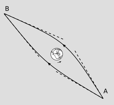
The astrophysical modeling of observations like figure d is complicated, but we can see in a simplified thought experiment that if we want to determine the angular momentum of a rotating body via its gravitational field, it will be difficult unless we use a measuring process that takes advantage of the asymptotic flatness of the space. For example, suppose we send two beams of light past the earth, in its equatorial plane, one on each side, and measure their deflections, e. The deflections will be different, because the sign of d\(\phi\) dt will be opposite for the two beams. But the entire notion of a “deflection” only makes sense if we have an asymptotically flat background, as indicated by the dashed tangent lines. Also, if spacetime were not asymptotically flat in this example, then there might be no unambiguous way to determine whether the asymmetry was due to the earth’s rotation, to some external factor, or to some kind of interaction between the earth and other bodies nearby.

Figure \(\PageIndex{5}\) - Two light rays travel in the earth’s equatorial plane from A to B. Due to frame-dragging, the ray moving with the earth’s rotation is deflected by a greater amount than the one moving contrary to it. As a result, the figure has an asymmetric banana shape. Both the deflection and its asymmetry are greatly exaggerated.

It also turns out that a gyroscope in such a gravitational field precesses. This effect, called frame dragging, was predicted by Lense and Thirring in 1918, and was finally verified experimentally in 2008 by analysis of data from the Gravity Probe B experiment, to a precision of about 15%. The experiment was arranged so that the relatively strong geodetic effect (6.6 arc-seconds per year) and the much weaker Lense-Thirring effect (.041 arc-sec/yr) produced precessions in perpendicular directions. Again, the presence of an asymptotically flat background was involved, because the probe measured the orientations of its gyroscopes relative to the guide star IM Pegasi.

Figure \(\PageIndex{6 }\) - Gravity Probe B verified the existence of frame-dragging. The rotational axis of the gyroscope precesses in two perpendicular planes due to the two separate effects: geodetic and frame-dragging.