5.6: Some Order-of-magnitude Estimates

As a general proposition, calculating an order-of-magnitude estimate of a physical effect requires an understanding of 50% of the physics, while an exact calculation requires about 75%.⁷ We’ve reached the point where it’s reasonable to attempt a variety of order-of-magnitude estimates.

Note

This statement is itself only a rough estimate. Anyone who has taught physics knows that students will often calculate an effect exactly while not understanding the underlying physics at all.

The Geodetic Effect

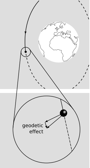
How could we confirm experimentally that parallel transport around a closed path can cause a vector to rotate? The rotation is related to the amount of spacetime curvature contained within the path, so it would make sense to choose a loop going around a gravitating body. The rotation is a purely relativistic effect, so we expect it to be small. To make it easier to detect, we should go around the loop many times, causing the effect to accumulate. This is essentially a description of a body orbiting another body. A gyroscope aboard the orbiting body is expected to precess. This is known as the geodetic effect. In 1916, shortly after Einstein published the general theory of relativity, Willem de Sitter calculated the effect on the earth-moon system. The effect was not directly verified until the 1980’s, and the first high-precision measurement was in 2007, from analysis of the results collected by the Gravity Probe B satellite experiment. The probe carried four gyroscopes made of quartz, which were the most perfect spheres ever manufactured, varying from sphericity by no more than about 40 atoms.

Figure \(\PageIndex{1}\) - The geodetic effect as measured by Gravity Probe B.

Let’s estimate the size of the effect. The first derivative of the metric is, roughly, the gravitational field, whereas the second derivative has to do with curvature. The curvature of spacetime around the earth should therefore vary as GMr⁻³, where M is the earth’s mass and G is the gravitational constant. The area enclosed by a circular orbit is proportional to r², so we expect the geodetic effect to vary as \(\frac{nGM}{r}\), where n is the number of orbits. The angle of precession is unitless, and the only way to make this result unitless is to put in a factor of \(\frac{1}{c^{2}}\). In units with c = 1, this factor is unnecessary. In ordinary metric units, the \(\frac{1}{c^{2}}\) makes sense, because it causes the purely relativistic effect to come out to be small. The result, up to unitless factors that we didn’t pretend to find, is

\[\Delta \theta \sim \frac{nGM}{c^{2} r} \ldotp\]

We might also expect a Thomas precession. Like the spacetime curvature effect, it would be proportional to \(\frac{nGM}{c^{2} r}\). Since we’re not worrying about unitless factors, we can just lump the Thomas precession together with the effect already calculated.

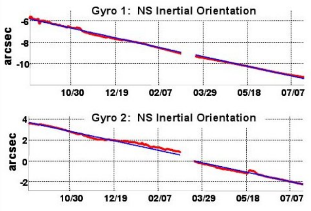
The data for Gravity Probe B are r = r_e+(650 km) and n ≈ 5000 (orbiting once every 90 minutes for the 353-day duration of the experiment), giving \(\Delta \theta\) ∼ 3 × 10⁻⁶ radians. Figure 5.5.2 shows the actual results⁸ the four gyroscopes aboard the probe. The precession was about 6 arc-seconds, or 3 × 10⁻⁵ radians. Our crude estimate was on the right order of magnitude. The missing unitless factor on the right-hand side of the equation above is 3\(\pi\), which brings the two results into fairly close quantitative agreement. The full derivation, including the factor of 3\(\pi\), is given in section 6.2.

Figure_5.5.2b.png" />

Figure \(\PageIndex{2}\) - Precession angle as a function of time as measured by the four gyroscopes aboard Gravity Probe B.

Deflection of Light Rays

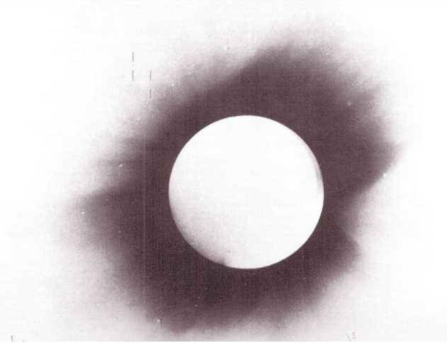
In the discussion of the momentum four vector in section 4.2, we saw that due to the equivalence principle, light must be affected by gravity. There are two ways in which such an effect could occur. Light can gain and lose momentum as it travels up and down in a gravitational field, or its momentum vector can be deflected by a transverse gravitational field. As an example of the latter, a ray of starlight can be deflected by the sun’s gravity, causing the star’s apparent position in the sky to be shifted. The detection of this effect was one of the first experimental tests of general relativity. Ordinarily the bright light from the sun would make it impossible to accurately measure a star’s location on the celestial sphere, but this problem was sidestepped by Arthur Eddington during an eclipse of the sun in 1919.

Let’s estimate the size of this effect. We’ve already seen that the Riemann tensor is essentially just a tensorial way of writing the Gaussian curvature \(K = \frac{d \epsilon}{dA}\). Suppose, for the sake of this rough estimate, that the sun, earth, and star form a non-Euclidean triangle with a right angle at the sun. Then the angular deflection is the same as the angular defect \(\epsilon\) of this triangle, and equals the integral of the curvature over the interior of the triangle. Ignoring unitless constants, this ends up being exactly the same calculation as earlier, and the result is \(\epsilon \sim \frac{GM}{c^{2} r}\), where r is the light ray’s distance of closest approach to the sun. The value of r can’t be less than the radius of the sun, so the maximum size of the effect is on the order of \(\frac{GM}{c^{2} r}\), where M is the sun’s mass, and \(r\) is its radius. We find \(\epsilon\) ∼ 10⁻⁵ radians, or about a second of arc. To measure a star’s position to within an arc second was well within the state of the art in 1919, under good conditions in a comfortable observatory. This observation, however, required that Eddington’s team travel to the island of Principe, off the coast of West Africa. The weather was cloudy, and only during the last 10 seconds of the seven-minute eclipse did the sky clear enough to allow photographic plates to be taken of the Hyades star cluster against the background of the eclipse-darkened sky. The observed deflection was 1.6 seconds of arc, in agreement with the relativistic prediction. The relativistic prediction is derived in section 6.2.

Figure \(\PageIndex{3}\) - One of the photos from Eddington’s observations of the 1919 eclipse. This is a photographic negative, so the circle that appears bright is actually the dark face of the moon, and the dark area is really the bright corona of the sun. The stars, marked by lines above and below them, appeared at positions slightly different than their normal ones, indicating that their light had been bent by the sun’s gravity on its way to our planet.

References

⁸ arxiv.org/abs/1105.3456