5.7: The Covariant Derivative

In the preceding section we were able to estimate a nontrivial general relativistic effect, the geodetic precession of the gyroscopes aboard Gravity Probe B, up to a unitless constant 3\(\pi\). Let’s think about what additional machinery would be needed in order to carry out the calculation in detail, including the 3\(\pi\).

First we would need to know the Einstein field equation, but in a vacuum this is fairly straightforward:

\[R_{ab} = 0.\]

Einstein posited this equation based essentially on the considerations laid out in Section 5.1.

But just knowing that a certain tensor vanishes identically in the space surrounding the earth clearly doesn’t tell us anything explicit about the structure of the spacetime in that region. We want to know the metric. As suggested at the beginning of the chapter, we expect that the first derivatives of the metric will give a quantity analogous to the gravitational field of Newtonian mechanics, but this quantity will not be directly observable, and will not be a tensor. The second derivatives of the metric are the ones that we expect to relate to the Ricci tensor \(R_{ab}\).

The Covariant Derivative in Electromagnetism

We’re talking blithely about derivatives, but it’s not obvious how to define a derivative in the context of general relativity in such a way that taking a derivative results in well-behaved tensor.

To see how this issue arises, let’s retreat to the more familiar terrain of electromagnetism. In quantum mechanics, the phase of a charged particle’s wavefunction is unobservable, so that for example the transformation \(\Psi \rightarrow − \Psi\) does not change the results of experiments. As a less trivial example, we can redefine the ground of our electrical potential, \(\Phi \rightarrow \Phi + \delta \Phi\), and this will add a constant onto the energy of every electron in the universe, causing their phases to oscillate at a greater rate due to the quantum-mechanical relation

\[E = hf.\]

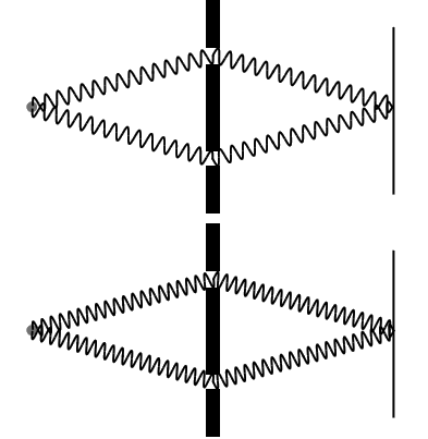
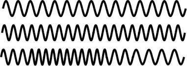
There are no observable consequences, however, because what is observable is the phase of one electron relative to another, as in a double-slit interference experiment. Since every electron has been made to oscillate faster, the effect is simply like letting the conductor of an orchestra wave her baton more quickly; every musician is still in step with every other musician. The rate of change of the wavefunction, i.e., its derivative, has some built-in ambiguity.

Figure \(\PageIndex{1}\) - A double-slit experiment with electrons. If we add an arbitrary constant to the potential, no observable changes result. The wavelength is shortened, but the relative phase of the two parts of the waves stays the same.

For simplicity, let’s now restrict ourselves to spin-zero particles, since details of electrons’ polarization clearly won’t tell us anything useful when we make the analogy with relativity. For a spin-zero particle, the wavefunction is simply a complex number, and there are no observable consequences arising from the transformation

\[\Psi \rightarrow \Psi' = e^{i \alpha} \Psi\]

where \(\alpha\) is a constant. The transformation \(\Phi \rightarrow \Phi + \delta \Phi\) is also allowed, and it gives \(\alpha (t) = (\frac{q \delta \Phi}{\hbar})t\), so that the phase factor e^{i\(\alpha\)(t)} is a function of time \(t\). Now from the point of view of electromagnetism in the age of Maxwell, with the electric and magnetic fields imagined as playing their roles against a background of Euclidean space and absolute time, the form of this time-dependent phase factor is very special and symmetrical; it depends only on the absolute time variable. But to a relativist, there is nothing very nice about this function at all, because there is nothing special about a time coordinate. If we’re going to allow a function of this form, then based on the coordinate-invariance of relativity, it seems that we should probably allow α to be any function at all of the spacetime coordinates. The proper generalization of \(\Phi \rightarrow \Phi - \delta \Phi\) is now A_b → A_b − \(\partial_{b} \alpha\), where A_b is the electromagnetic potential four-vector (section 4.2).

Figure \(\PageIndex{2}\) - Two wavefunctions with constant wavelengths, and a third with a varying wavelength. None of these are physically distinguishable, provided that the same variation in wavelength is applied to all electrons in the universe at any given point in spacetime. There is not even any unambiguous way to pick out the third one as the one with a varying wavelength. We could choose a different gauge in which the third wave was the only one with a constant wavelength.

Exercise \(\PageIndex{1}\)

Self-check: Suppose we said we would allow \(\alpha\) to be a function of t, but forbid it to depend on the spatial coordinates. Prove that this would violate Lorentz invariance.

The transformation has no effect on the electromagnetic fields, which are the direct observables. We can also verify that the change of gauge will have no effect on observable behavior of charged particles. This is because the phase of a wavefunction can only be determined relative to the phase of another particle’s wavefunction, when they occupy the same point in space and, for example, interfere. Since the phase shift depends only on the location in spacetime, there is no change in the relative phase.

But bad things will happen if we don’t make a corresponding adjustment to the derivatives appearing in the Schrödinger equation. These derivatives are essentially the momentum operators, and they give different results when applied to \(\Psi'\) than when applied to \(\Psi\):

\[\begin{split} \partial_{b} \Psi &\rightarrow \partial_{b} (e^{i \alpha} \Psi) \\ &= e^{i \alpha} \partial_{b} \Psi + i \partial_{b} \alpha (e^{i \alpha} \Psi) \\ &= (\partial_{b} + A'_{b} - A_{b}) \Psi' \end{split}\]

To avoid getting incorrect results, we have to do the substitution \(\partial_{b} \rightarrow \partial_{b} + ieA_{b}\), where the correction term compensates for the change of gauge. We call the operator \(\nabla\) defined as

\[\nabla_{b} = \partial_{b} + ieA_{b}\]

the covariant derivative. It gives the right answer regardless of a change of gauge.

The Covariant Derivative in General Relativity

Now consider how all of this plays out in the context of general relativity. The gauge transformations of general relativity are arbitrary smooth changes of coordinates. One of the most basic properties we could require of a derivative operator is that it must give zero on a constant function. A constant scalar function remains constant when expressed in a new coordinate system, but the same is not true for a constant vector function, or for any tensor of higher rank. This is because the change of coordinates changes the units in which the vector is measured, and if the change of coordinates is nonlinear, the units vary from point to point.

Figure \(\PageIndex{2}\) switching from one set of coordinates to another has no effect on any experimental observables. It is merely a choice of gauge.

Consider the one-dimensional case, in which a vector v^a has only one component, and the metric is also a single number, so that we can omit the indices and simply write v and g. (We just have to remember that v is really a covariant vector, even though we’re leaving out the upper index.) If v is constant, its derivative \(\frac{dv}{dx}\), computed in the ordinary way without any correction term, is zero. If we further assume that the coordinate x is a normal coordinate, so that the metric is simply the constant g = 1, then zero is not just the answer but the right answer. (The existence of a preferred, global set of normal coordinates is a special feature of a one-dimensional space, because there is no curvature in one dimension. In more than one dimension, there will typically be no possible set of coordinates in which the metric is constant, and normal coordinates only give a metric that is approximately constant in the neighborhood around a certain point. See Figure 5.3.7 for an example of normal coordinates on a sphere, which do not have a constant metric.)

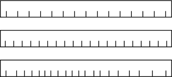
Now suppose we transform into a new coordinate system X, which is not normal. The metric G, expressed in this coordinate system, is not constant. Applying the tensor transformation law, we have \(V = v \frac{dX}{dx}\), and differentiation with respect to X will not give zero, because the factor \(\frac{dX}{dx}\) isn’t constant. This is the wrong answer: V isn’t really varying, it just appears to vary because G does.

We want to add a correction term onto the derivative operator \(\frac{d}{dX}\), forming a covariant derivative operator \(\nabla_{X}\) that gives the right answer. This correction term is easy to find if we consider what the result ought to be when differentiating the metric itself. In general, if a tensor appears to vary, it could vary either because it really does vary or because the metric varies. If the metric itself varies, it could be either because the metric really does vary or . . . because the metric varies. In other words, there is no sensible way to assign a nonzero covariant derivative to the metric itself, so we must have \(\nabla_{X}\)G = 0. The required correction therefore consists of replacing \(\frac{d}{dX}\) with

\[\nabla_{X} = \frac{d}{dX} - G^{-1} \frac{dG}{dX} \ldotp\]

Applying this to G gives zero. G is a second-rank contravariant tensor. If we apply the same correction to the derivatives of other second-rank contravariant tensors, we will get nonzero results, and they will be the right nonzero results. For example, the covariant derivative of the stress-energy tensor T (assuming such a thing could have some physical significance in one dimension!) will be \(\nabla_{X} T = \frac{dT}{dX} − G^{-1} (\frac{dG}{dX})T\).

Physically, the correction term is a derivative of the metric, and we’ve already seen that the derivatives of the metric (1) are the closest thing we get in general relativity to the gravitational field, and (2) are not tensors. In 1+1 dimensions, suppose we observe that a free-falling rock has \(\frac{dV}{dT}\) = 9.8 m/s². This acceleration cannot be a tensor, because we could make it vanish by changing from Earthfixed coordinates X to free-falling (normal, locally Lorentzian) coordinates x, and a tensor cannot be made to vanish by a change of coordinates. According to a free-falling observer, the vector v isn’t changing at all; it is only the variation in the Earth-fixed observer’s metric G that makes it appear to change.

Mathematically, the form of the derivative is \((\frac{1}{y}) \frac{dy}{dx}\), which is known as a logarithmic derivative, since it equals \(\frac{d(\ln y)}{dx}\). It measures the multiplicative rate of change of y. For example, if y scales up by a factor of k when x increases by 1 unit, then the logarithmic derivative of y is ln k. The logarithmic derivative of e^cx is c. The logarithmic nature of the correction term to \(\nabla_{X}\) is a good thing, because it lets us take changes of scale, which are multiplicative changes, and convert them to additive corrections to the derivative operator. The additivity of the corrections is necessary if the result of a covariant derivative is to be a tensor, since tensors are additive creatures.

What about quantities that are not second-rank covariant tensors? Under a rescaling of contravariant coordinates by a factor of k, covariant vectors scale by k⁻¹, and second-rank covariant tensors by k⁻². The correction term should therefore be half as much for covariant vectors,

\[\nabla_{X} = \frac{d}{dX} - \frac{1}{2} G^{-1} \frac{dG}{dX} \ldotp\]

and should have an opposite sign for contravariant vectors.

Generalizing the correction term to derivatives of vectors in more than one dimension, we should have something of this form:

\[\begin{split} \nabla_{a} v^{b} &= \partial_{a} v^{b} + \Gamma^{b}_{ac} v^{c} \\ \nabla_{a} v_{b} &= \partial_{a} v_{b} - \Gamma^{c}_{ba} v_{c}, \end{split}\]

where \(\Gamma^{b}_{ac}\), called the Christoffel symbol, does not transform like a tensor, and involves derivatives of the metric. (“Christoffel” is pronounced “Krist-AWful,” with the accent on the middle syllable.) The explicit computation of the Christoffel symbols from the metric is deferred until section 5.9, but the intervening sections 5.7 and 5.8 can be omitted on a first reading without loss of continuity.

An important gotcha is that when we evaluate a particular component of a covariant derivative such as \(\nabla_{2} v^{3}\), it is possible for the result to be nonzero even if the component v³ vanishes identically. This can be seen in example 5 and example 21.

Example 9: Christoffel symbols on the globe

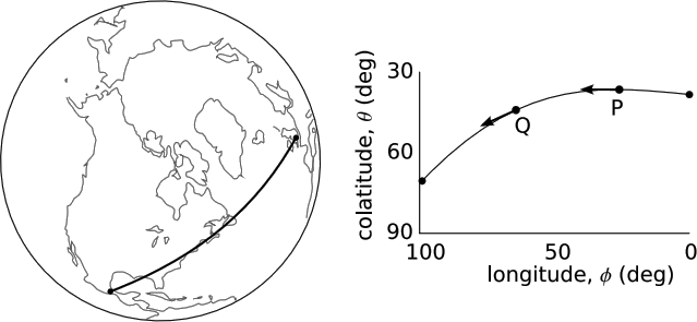
As a qualitative example, consider the geodesic airplane trajectory shown in Figure 5.6.4, from London to Mexico City. In physics it is customary to work with the colatitude, \(\theta\), measured down from the north pole, rather then the latitude, measured from the equator. At P, over the North Atlantic, the plane’s colatitude has a minimum. (We can see, without having to take it on faith from the figure, that such a minimum must occur. The easiest way to convince oneself of this is to consider a path that goes directly over the pole, at \(\theta\) = 0.)

Figure \(\PageIndex{4}\)

At P, the plane’s velocity vector points directly west. At Q, over New England, its velocity has a large component to the south. Since the path is a geodesic and the plane has constant speed, the velocity vector is simply being parallel-transported; the vector’s covariant derivative is zero. Since we have v_\(\theta\) = 0 at P, the only way to explain the nonzero and positive value of \(\partial_{\phi} v^{\theta}\) is that we have a nonzero and negative value of \(\Gamma^{\theta}_{\phi \phi}\).

By symmetry, we can infer that \(\Gamma^{\theta}_{\phi \phi}\) must have a positive value in the southern hemisphere, and must vanish at the equator.

\(\Gamma^{\theta}_{\phi \phi}\) is computed in example 10.

Symmetry also requires that this Christoffel symbol be independent of \(\phi\), and it must also be independent of the radius of the sphere.

Example 9 is in two spatial dimensions. In spacetime, \(\Gamma\) is essentially the gravitational field (see problem 7), and early papers in relativity essentially refer to it that way.⁹ This may feel like a joyous reunion with our old friend from freshman mechanics, g = 9.8 m/s. But our old friend has changed. In Newtonian mechanics, accelerations like g are frame-invariant (considering only inertial frames, which are the only legitimate ones in that theory). In general relativity they are frame-dependent, and as we saw earlier, the acceleration of gravity can be made to equal anything we like, based on our choice of a frame of reference.

To compute the covariant derivative of a higher-rank tensor, we just add more correction terms, e.g.,

\[\nabla_{a} U_{bc} = \partial_{a} U_{bc} - \Gamma^{d}_{ba} U_{dc} - \Gamma^{d}_{ca} U_{bd}\]

or

\[\nabla_{a} U_{b}^{c} = \partial_{a} U_{b}^{c} - \Gamma^{d}_{ba} U_{d}^{c} + \Gamma^{c}_{ad} U_{b}^{d} \ldotp\]

With the partial derivative \(\partial_{\mu}\), it does not make sense to use the metric to raise the index and form \(\partial^{\mu}\). It does make sense to do so with covariant derivatives, so \(\nabla^{a} = g^{ab} \nabla_{b}\) is a correct identity.

Comma, Semicolon, and Birdtracks Notation

Some authors use superscripts with commas and semicolons to indicate partial and covariant derivatives. The following equations give equivalent notations for the same derivatives:

\[\partial_{\mu} X_{\nu} = X_{\nu,\; \mu}\]

\[\nabla_{a} X_{b} = X_{b;a}\]

\[\nabla^{a} X_{b} = X_{b}^{;a}\]

Figure 5.6.5 shows two examples of the corresponding birdtracks notation. Because birdtracks are meant to be manifestly coordinate-independent, they do not have a way of expressing non-covariant derivatives. We no longer want to use the circle as a notation for a non-covariant gradient as we did when we first introduced it in section 2.1.

References

⁹ “On the gravitational field of a point mass according to Einstein’s theory,” Sitzungsberichte der Königlich Preussischen Akademie der Wissenschaften 1 (1916) 189, translated in arxiv.org/abs/physics/9905030v1.