8.2: Sources in General Relativity (Part 2)

Energy of Gravitational Fields Not Included in the Stress-energy Tensor

Summarizing the story of the Kreuzer and Bartlett-van Buren results, we find that observations verify to high precision one of the defining properties of general relativity, which is that all forms of energy are equivalent to mass. That is, Einstein’s famous E = mc² can be extended to gravitational effects, with the proviso that the source of gravitational fields is not really a scalar m but the stressenergy tensor T.

But there is an exception to this even-handed treatment of all types of energy, which is that the energy of the gravitational field itself is not included in T, and is not even generally a well-defined concept locally. In Newtonian gravity, we can have conservation of energy if we attribute to the gravitational field a negative potential energy density \(− \frac{\textbf{g}^{2}}{8 \pi}\). But the equivalence principle tells us that g is not a tensor, for we can always make g vanish locally by going into the frame of a free-falling observer, and yet the tensor transformation laws will never change a nonzero tensor to a zero tensor under a change of coordinates. Since the gravitational field is not a tensor, there is no way to add a term for it into the definition of the stress-energy, which is a tensor. The grammar and vocabulary of the tensor notation are specifically designed to prevent writing down such a thing, so that the language of general relativity is not even capable of expressing the idea that gravitational fields would themselves contribute to T.

exercise \(\PageIndex{2}\)

Self-check: (1) Convince yourself that the negative sign in the expression \(− \frac{\textbf{g}^{2}}{8 \pi}\) makes sense, by considering the case where two equal masses start out far apart and then fall together and combine to make a single body with twice the mass. (2) The Newtonian gravitational field is the gradient of the gravitational potential \(\phi\), which corresponds in the Newtonian limit to the time-time component of the metric. With this motivation, suppose someone proposes generalizing the Newtonian energy density \(− \frac{(\nabla \phi)^{2}}{8 \pi}\) to a similar expression such as \(−(\nabla_{a} g^{a}_{b})(\nabla_{c} g^{b}_{c})\), where \(\nabla\) is now the covariant derivative, and g is the metric, not the Newtonian field strength. What goes wrong?

As a concrete example, we observe that the Hulse-Taylor binary pulsar system (section 6.2) is gradually losing orbital energy, and that the rate of energy loss exactly matches general relativity’s prediction of the rate of gravitational radiation. There is a net decrease in the forms of energy, such as rest mass and kinetic energy, that are accounted for in the stress energy tensor T. We can account for the missing energy by attributing it to the outgoing gravitational waves, but that energy is not included in T, and we have to develop special techniques for evaluating that energy. Those techniques only turn out to apply to certain special types of spacetimes, such as asymptotically flat ones, and they do not allow a uniquely defined energy density to be attributed to a particular small region of space (for if they did, that would violate the equivalence principle).

Example 3: Gravitational energy is locally unmeasurable

When a new form of energy is discovered, the way we establish that it is a form of energy is that it can be transformed to or from other forms of energy. For example, Becquerel discovered radioactivity by noticing that photographic plates left in a desk drawer along with radium salts became clouded: some new form of energy had been converted into previously known forms such as chemical energy. It is only in this limited sense that energy is ever locally observable, and this limitation prevents us from meaningfully defining certain measures of energy. For example we can never measure the local electrical potential in the same sense that we can measure the local barometric pressure; a potential of 137 volts only has meaning relative to some other region of space taken to be at ground. Let’s use the acronym MELT to refer to measurement of energy by the local transformation of that energy from one form into another.

The reason MELT works is that energy (or actually the momentum four-vector) is locally conserved, as expressed by the zerodivergence property of the stress-energy tensor. Without conservation, there is no notion of transformation. The Einstein field equations imply this zero-divergence property, and the field equations have been well verified by a variety of observations, including many observations (such as solar system tests and observation of the Hulse-Taylor system) that in Newtonian terms would be described as involving (non-local) transformations between kinetic energy and the energy of the gravitational field. This agreement with observation is achieved by taking T = 0 in vacuum, regardless of the gravitational field. Therefore any local transformation of gravitational field energy into another form of energy would be inconsistent with previous observation. This implies that MELT is impossible for gravitational field energy.

In particular, suppose that observer A carries out a local MELT of gravitational field energy, and that A sees this as a process in which the gravitational field is reduced in intensity, causing the release of some other form of energy such as heat. Now consider the situation as seen by observer B, who is free-falling in the same local region. B says that there was never any gravitational field in the first place, and therefore sees heat as violating local conservation of energy. In B’s frame, this is a nonzero divergence of the stress-energy tensor, which falsifies the Einstein field equations.

Some Examples

We conclude this introduction to the stress-energy tensor with some illustrative examples.

Example 4: A perfect fluid

For a perfect fluid, we have $$T_{ab} = (\rho + P) v_{a} v_{b} - sPg_{ab}, \tag{8.1.11}\]

where s = 1 for our + − −− signature or −1 for the signature − + ++, and v represents the coordinate velocity of the fluid’s rest frame.

Suppose that the metric is diagonal, but its components are varying, g_{\(\alpha \beta\)} = diag(A², −B², . . .). The properly normalized velocity vector of an observer at (coordinate-)rest is v^\(\alpha\) = (A⁻¹, 0, 0, 0). Lowering the index gives v_\(\alpha\) = (sA, 0, 0, 0). The various forms of the stress-energy tensor then look like the following:

\[\begin{split} T_{00} &= A^{2} \rho \qquad \; \; \; T_{11} = B^{2} P \\ T^{0}_{0} &= s \rho \qquad \quad \; \; T^{1}_{1} = -sP \\ T^{00} &= A^{-2} \rho \qquad T^{11} = B^{-2} P \ldotp \end{split}\]

Example 5: A rope dangling in a Schwarzschild spacetime

Suppose we want to lower a bucket on a rope toward the event horizon of a black hole. We have already made some qualitative remarks about this idea in example 14 on p. 64. This seemingly whimsical example turns out to be a good demonstration of some techniques, and can also be used in thought experiments that illustrate the definition of mass in general relativity and that probe some ideas about quantum gravity.⁵

The Schwarzschild metric (section 6.2) is

\[ds^{2} = t^{2} dt^{2} - t^{-2} dr^{2} + \ldots, \tag{8.1.12}\]

where f = (1 − \f(\frac{2m}{r}\))^1/2, and . . . represents angular terms. We will end up needing the following Christoffel symbols:

\[\begin{split} \Gamma^{t}_{tr} &= \frac{f'}{f} \\ \Gamma^{\theta}_{\theta r} &= \Gamma^{\phi}_{\phi r} = r^{-1} \end{split}\]

Since the spacetime has spherical symmetry, it ends up being more convenient to consider a rope whose shape, rather than being cylindrical, is a cone defined by some set of \((\theta, \phi)\). For convenience we take this set to cover unit solid angle. The final results obtained in this way can be readily converted into statements about a cylindrical rope. We let µ be the mass per unit length of the rope, and T the tension. Both of these may depend on r. The corresponding energy density and tensile stress are \(\rho = \frac{\mu}{A} = \frac{\mu}{r^{2}}\) and S = \(\frac{T}{A}\). To connect this to the stress-energy tensor, we start by comparing to the case of a perfect fluid from example 4. Because the rope is made of fibers that have stength only in the radial direction, we will have T^{\(\theta \theta\)} = T^{\(\phi \phi\)} = 0. Furthermore, the stress is tensile rather than compressional, corresponding to a negative pressure. The Schwarzschild coordinates are orthogonal but not orthonormal, so the properly normalized velocity of a static observer has a factor of f in it: v^\(\alpha\) = (f⁻¹, 0, 0, 0), or, lowering an index, v_\(\alpha\) = (f, 0, 0, 0). The results of example 4 show that the mixed-index form of T will be the most convenient, since it can be expressed without messy factors of f. We have

\[T^{\kappa}_{\nu} = diag(\rho, S, 0, 0) = r^{-2} diag(\mu, T, 0, 0) \ldotp \tag{8.1.13}\]

By writing the stress-energy tensor in this form, which is independent of t, we have assumed static equilibrium outside the event horizon. Inside the horizon, the r coordinate is the timelike one, the spacetime itself is not static, and we do not expect to find static solutions, for the reasons given in example 14.

Conservation of energy is automatically satisfied, since there is no time dependence. Conservation of radial momentum is expressed by

\[\nabla_{\kappa} T^{\kappa}_{r} = 0, \tag{8.1.14}\]

or

\[0 = \nabla_{r} T^{r}_{r} + \nabla_{t} T^{t}_{r} + \nabla_{\theta} T^{\theta}_{r} + \nabla_{\phi} T^{\phi}_{r} \ldotp \tag{8.1.15}\]

It would be tempting to throw away all but the first term, since T is diagonal, and therefore \(T^{t}_{r} = T^{\theta}_{r} = T^{\phi}_{r} = 0\). However, a covariant derivative can be nonzero even when the symbol being differentiated vanishes identically. Writing out these four terms, we have

\[\begin{split} 0 &= \partial_{r} T^{r}_{r} + \Gamma^{r}_{rr} T^{r}_{r} - \Gamma^{r}_{rr} T^{r}_{r} \\ &+ \Gamma^{t}_{tr} T^{r}_{r} - \Gamma^{t}_{tr} T^{t}_{t} \\ &+ \Gamma^{\theta}_{\theta r} T^{r}_{r} \\ &+ \Gamma^{\phi}_{\phi r} T^{r}_{r}, \end{split}\]

where each line corresponds to one covariant derivative. Evaluating this, we have

\[0 = T' + \frac{f'}{f} T - \frac{f'}{f} \mu, \tag{8.1.16}\]

where primes denote differentiation with respect to r. Note that since no terms of the form \(\partial_{r} T^{t}_{t}\) occur, this expression is valid regardless of whether we take µ to be constant or varying. Thus we are free to take \(\rho \propto r^{−2}\), so that \(\mu\) is constant, and this means that our result is equally applicable to a uniform cylindrical rope. This result is checked using computer software in example 6.

This is a differential equation that tells us how the tensile stress in the rope varies along its length. The coefficient \(\frac{f'}{f} = \frac{m}{r(r −2m)}\) blows up at the event horizon, which is as expected, since we do not expect to be able to lower the rope to or below the horizon.

Let’s check the Newtonian limit, where the gravitational field is g and the potential is \(\Phi\). In this limit, we have f ≈ 1 − \(\Phi\), \(\frac{f'}{f}\) ≈ g (with g > 0), and \(\mu\) >> T, resulting in

\[0 = T' - g \mu \ldotp \tag{8.1.17}\]

which is the expected Newtonian relation.

Returning to the full general-relativistic result, it can be shown that for a loaded rope with no mass of its own, we have a finite result for \(lim_{r \rightarrow \infty}\) T, even when the bucket is brought arbitrarily close to the horizon. (The solution in this case is just T = \(\frac{T_{\infty}}{f}\), where T_∞ is the tension at r = ∞.) However, this is misleading without the caveat that for \(\mu\) < T, the speed of transverse waves in the rope is greater than c, which is not possible for any known form of matter — it would violate the null energy condition, discussed in the following section.

---

⁵ Brown, “Tensile Strength and the Mining of Black Holes,” arxiv.org/abs/ 1207.3342

Example 6: The rope, using computer algebra

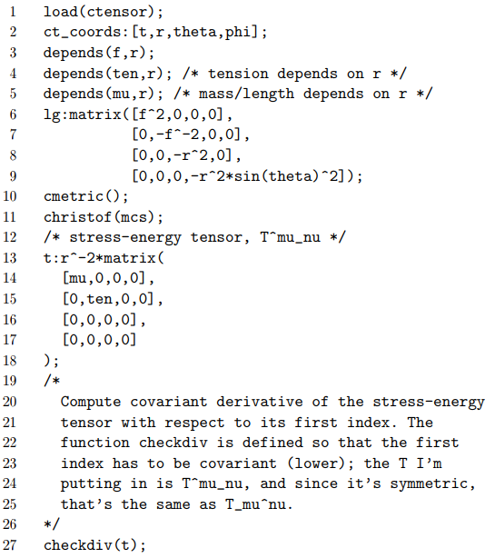
The result of example 5 can be checked with the following Maxima code:

Energy Conditions

Physical theories are supposed to answer questions. For example:

1. Does a small enough physical object always have a world-line that is approximately a geodesic?
2. Do massive stars collapse to form black-hole singularities?
3. Did our universe originate in a Big Bang singularity?
4. If our universe doesn’t currently have violations of causality such as the closed timelike curves exhibited by the Petrov metric (section 7.5), can we be assured that it will never develop causality violation in the future?

We would like to “prove” whether the answers to questions like these are yes or no, but physical theories are not formal mathematical systems in which results can be “proved” absolutely. For example, the basic structure of general relativity isn’t a set of axioms but a list of ingredients like the equivalence principle, which has evaded formal definition.⁶

Even the Einstein field equations, which appear to be completely well defined, are not mathematically formal predictions of the behavior of a physical system. The field equations are agnostic on the question of what kinds of matter fields contribute to the stress-energy tensor. In fact, any spacetime at all is a solution to the Einstein field equations, provided we’re willing to admit the corresponding stress-energy tensor. We can never answer questions like the ones above without assuming something about the stress-energy tensor.

In example 14, we saw that radiation has P = \(\frac{\rho}{3}\) and dust has P = 0. Both have \(\rho\) ≥ 0. If the universe is made out of nothing but dust and radiation, then we can obtain the following four constraints on the energy-momentum tensor:

trace energy condition	\(\rho - 3P \geq 0\)
strong energy condition	\(\rho + 3P \geq 0\; and\; \rho + P \geq 0\)
dominant energy condition	\(\rho \geq 0\; and\; |P| \leq \rho\)
weak energy condition	\(\rho \geq 0\; and\; \rho + P \geq 0\)
null energy condition	\(\rho + P \geq 0\)

These are arranged roughly in order from strongest to weakest. They all have to do with the idea that negative mass-energy doesn’t seem to exist in our universe, i.e., that gravity is always attractive rather than repulsive. With this motivation, it would seem that there should only be one way to state an energy condition: \(\rho\) > 0. But the symbols \(\rho\) and P refer to the form of the stress-energy tensor in a special frame of reference, interpreted as the one that is at rest relative to the average motion of the ambient matter. (Such a frame is not even guaranteed to exist unless the matter acts as a perfect fluid.) In this frame, the tensor is diagonal. Switching to some other frame of reference, the \(\rho\) and P parts of the tensor would mix, and it might be possible to end up with a negative energy density. The weak energy condition is the constraint we need in order to make sure that the energy density is never negative in any frame.

The dominant energy condition is like the weak energy condition, but it also guarantees that no observer will see a flux of energy flowing at speeds greater than c.

The strong energy condition essentially states that gravity is never repulsive; it is violated by the cosmological constant (see section 8.2).

Example 7: An electromagnetic wave

In example 1, we saw that dust boosted along the x axis gave a stress-energy tensor

\[T_{\mu \nu} = \gamma^{2} \rho \begin{pmatrix} 1 & v \\ v & v^{2} \end{pmatrix}, \tag{8.1.18}\]

where we now suppress the y and z parts, which vanish. For v → 1, this becomes

\[T_{\mu \nu} = \rho' \begin{pmatrix} 1 & 1 \\ 1 & 1 \end{pmatrix}, \tag{8.1.19}\]

where \(\rho'\) is the energy density as measured in the new frame. As a source of gravitational fields, this ultrarelativistic dust is indistinguishable from any other form of matter with v = 1 along the x axis, so this is also the stress-energy tensor of an electromagnetic wave with local energy-density ρ 0 , propagating along the x axis. (For the full expression for the stress-energy tensor of an arbitrary electromagnetic field, see the Wikipedia article “Electromagnetic stress-energy tensor.”)

This is a stress-energy tensor that represents a flux of energy at a speed equal to c, so we expect it to lie at exactly the limit imposed by the dominant energy condition (DEC). Our statement of the DEC, however, was made for a diagonal stress-energy tensor, which is what is seen by an observer at rest relative to the matter. But we know that it’s impossible to have an observer who, as the teenage Einstein imagined, rides alongside an electromagnetic wave on a motorcycle. One way to handle this is to generalize our definition of the energy condition. For the DEC, it turns out that this can be done by requiring that the matrix T, when multiplied by a vector on or inside the future light-cone, gives another vector on or inside the cone.

A less elegant but more concrete workaround is as follows. Returning to the original expression for the T of boosted dust at velocity v, we let v = 1 + \(\epsilon\), where |\(\epsilon\)| << 1. This gives a stress-energy tensor that (ignoring multiplicative constants) looks like:

\[\begin{pmatrix} 1 & 1 + \epsilon \\ 1 + \epsilon & 1 + 2 \epsilon \end{pmatrix} \ldotp \tag{8.1.20}\]

If \(\epsilon\) is negative, we have ultrarelativistic dust, and we can verify that it satisfies the DEC by un-boosting back to the rest frame. To do this explicitly, we can find the matrix’s eigenvectors, which (ignoring terms of order \(\epsilon^{2}\)) are (1, 1 + \(\epsilon\)) and (1, 1 − \(\epsilon\)), with eigenvalues 2 + 2\(\epsilon\) and 0, respectively. For \(\epsilon\) < 0, the first of these is timelike, the second spacelike. We interpret them simply as the t and x basis vectors of the rest frame in which we originally described the dust. Using them as a basis, the stress-energy tensor takes on the form diag(2 + 2\(\epsilon\), 0). Except for a constant factor that we didn’t bother to keep track of, this is the original form of the T in the dust’s rest frame, and it clearly satisfies the DEC, since P = 0.

For \(\epsilon\) > 0, v = 1 + \(\epsilon\) is a velocity greater than the speed of light, and there is no way to construct a boost corresponding to −v. We can nevertheless find a frame of reference in which the stressenergy tensor is diagonal, allowing us to check the DEC. The expressions found above for the eigenvectors and eigenvalues are still valid, but now the timelike and spacelike characters of the two basis vectors have been interchanged. The stress-energy tensor has the form diag(0, 2 + 2\(\epsilon\)), with \(\rho\) = 0 and P > 0, which violates the DEC. As in this example, any flux of mass-energy at speeds greater than c will violate the DEC.

The DEC is obeyed for \(\epsilon\) < 0 and violated for \(\epsilon\) > 0, and since \(\epsilon\) = 0 gives a stress-energy tensor equal to that of an electromagnetic wave, we can tell that light is exactly on the border between forms of matter that fulfill the DEC and those that don’t. Since the DEC is formulated as a non-strict inequality, it follows that light obeys the DEC.

Example 8: No “speed of flux”

The foregoing discussion may have encouraged the reader to believe that it is possible in general to read off a “speed of energy flux” from the value of T at a point. This is not true.

The difficulty lies in the distinction between flow with and without accumulation, which is sometimes valid and sometimes not. In springtime in the Sierra Nevada, snowmelt adds water to alpine lakes more rapidly than it can flow out, and the water level rises. This is flow with accumulation. In the fall, the reverse happens, and we have flow with depletion (negative accumulation).

Figure 8.1.5 (1) shows a second example in which the distinction seems valid. Charge is flowing through the lightbulb, but because there is no accumulation of charge in the DC circuit, we can’t detect the flow by an electrostatic measurement; the wire does not attract the tiny bits of paper below it on the table.

But we know that with different measurements, we could detect the flow of charge in Figure 8.1.5 (1). For example, the magnetic field from the wire would deflect a nearby magnetic compass. This shows that the distinction between flow with and without accumulation may be sometimes valid and sometimes invalid. Flow without accumulation may or may not be detectable; it depends on the physical context.

In Figure 8.1.5 (2), an electric charge and a magnetic dipole are super-imposed at a point. The Poynting vector P defined as E × B is used in electromagnetism as a measure of the flux of energy, and it tells the truth, for example, when the sun warms your sun on a hot day. In Figure 8.1.5 (2), however, all the fields are static. It seems as though there can be no flux of energy. But that doesn’t mean that the Poynting vector is lying to us. It tells us that there is a pattern of flow, but it’s flow without accumulation; the Poynting vector forms circular loops that close upon themselves, and electromagnetic energy is transported in and out of any volume at the same rate. We would perhaps prefer to have a mathematical rule that gave zero for the flux in this situation, but it’s acceptable that our rule P = E × B gives a nonzero result, since it doesn’t incorrectly predict an accumulation, which is what would be detectable.

Figure_8.1.5b.png" />

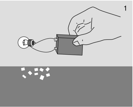
Figure \(\PageIndex{5}\)

Now suppose we’re presented with this stress-energy tensor, measured at a single point and expressed in some units:

\[T^{\mu \nu} = \begin{pmatrix} 4.037 \pm 0.002 & 4.038 \pm 0.002 \\ 4.036 \pm 0.002 & 4.036 \pm 0.002 \end{pmatrix} \ldotp \tag{8.1.21}\]

To within the experimental error bars, it has the right form to be many different things: (1) We could have a universe filled with perfectly uniform dust, moving along the x axis at some ultrarelativistic speed v so great that the \(\epsilon\) in v = 1 − \(\epsilon\), as in example 7, is not detectably different from zero. (2) This could be a point sampled from an electromagnetic wave traveling along the x axis. (3) It could be a point taken from Figure 8.1.5 (2). (In cases 2 and 3, the off-diagonal elements are simply the Poynting vector.)

In cases 1 and 2, we would be inclined to interpret this stress-energy tensor by saying that its off-diagonal part measures the flux of mass-energy along the x axis, while in case 3 we would reject such an interpretation. The trouble here is not so much in our interpretation of T as in our Newtonian expectations about what is or isn’t observable about fluxes that flow without accumulation. In Newtonian mechanics, a flow of mass is observable, regardless of whether there is accumulation, because it carries momentum with it; a flow of energy, however, is undetectable if there is no accumulation. The trouble here is that relativistically, we can’t maintain this distinction between mass and energy. The Einstein field equations tell us that a flow of either will contribute equally to the stress-energy, and therefore to the surrounding gravitational field.

The flow of energy in Figure 8.1.5 (2) contributes to the gravitational field, and its contribution is changed, for example, if the magnetic field is reversed. The figure is in fact not a bad qualitative representation of the spacetime around a rotating, charged black hole. At large distances, however, the gravitational effect of the off-diagonal terms in T becomes small, because they average to nearly zero over a sufficiently large spherical region. The distant gravitational field approaches that of a point mass with the same mass-energy

Example 9: Momentum in static fields

Continuing the train of thought described in example 8, we can come up with situations that seem even more paradoxical. In Figure 8.1.5 (2), the total momentum of the fields vanishes by symmetry. This symmetry can, however, be broken by displacing the electric charge by ∆R perpendicular to the magnetic dipole vector D. The total momentum no longer vanishes, and now lies in the direction of D × ∆R. But we have proved in example 2 that a system’s center of mass-energy is at rest if and only if its total momentum is zero. Since this system’s center of mass-energy is certainly at rest, where is the other momentum that cancels that of the electric and magnetic fields?

Suppose, for example, that the magnetic dipole consists of a loop of copper wire with a current running around it. If we open a switch and extinguish the dipole, it appears that the system must recoil! This seems impossible, since the fields are static, and an electric charge does not interact with a magnetic dipole.

Babson et al.⁷ have analyzed a number of examples of this type. In the present one, the mysterious “other momentum” can be attributed to a relativistic imbalance between the momenta of the electrons in the different parts of the wire. A subtle point about these examples is that even in the case of an idealized dipole of vanishingly small size, it makes a difference what structure we assume for the dipole. In particular, the field’s momentum is nonzero for a dipole made from a current loop of infinitesimal size, but zero for a dipole made out of two magnetic monopoles.⁸

---

⁷ Am. J. Phys. 77 (2009) 826

⁸ Milton and Meille, arxiv.org/abs/1208.4826

References

⁶ “Theory of gravitation theories: a no-progress report,” Sotiriou, Faraoni, and Liberati, http://arxiv.org/abs/0707.2748