8.1: Sources in General Relativity (Part 1)

Point Sources in a Background-independent Theory

The Schrödinger equation and Maxwell’s equations treat spacetime as a stage on which particles and fields act out their roles. General relativity, however, is essentially a theory of spacetime itself. The role played by atoms or rays of light is so peripheral that by the time Einstein had derived an approximate version of the Schwarzschild metric, and used it to find the precession of Mercury’s perihelion, he still had only vague ideas of how light and matter would fit into the picture. In his calculation, Mercury played the role of a test particle: a lump of mass so tiny that it can be tossed into spacetime in order to measure spacetime’s curvature, without worrying about its effect on the spacetime, which is assumed to be negligible. Likewise the sun was treated as in one of those orchestral pieces in which some of the brass play from off-stage, so as to produce the effect of a second band heard from a distance. Its mass appears simply as an adjustable parameter m in the metric, and if we had never heard of the Newtonian theory we would have had no way of knowing how to interpret m.

When Schwarzschild published his exact solution to the vacuum field equations, Einstein suffered from philosophical indigestion. His strong belief in Mach’s principle led him to believe that there was a paradox implicit in an exact spacetime with only one mass in it. If Einstein’s field equations were to mean anything, he believed that they had to be interpreted in terms of the motion of one body relative to another. In a universe with only one massive particle, there would be no relative motion, and so, it seemed to him, no motion of any kind, and no meaningful interpretation for the surrounding spacetime.

Not only that, but Schwarzschild’s solution had a singularity at its center. When a classical field theory contains singularities, Einstein believed, it contains the seeds of its own destruction. As we’ve seen in section 6.3, this issue is still far from being resolved, a century later.

However much he might have liked to disown it, Einstein was now in possession of a solution to his field equations for a point source. In a linear, background-dependent theory like electromagnetism, knowledge of such a solution leads directly to the ability to write down the field equations with sources included. If Coulomb’s law tells us the \(\frac{1}{r^{2}}\) variation of the electric field of a point charge, then we can infer Gauss’s law. The situation in general relativity is not this simple. The field equations of general relativity, unlike the Gauss’s law, are nonlinear, so we can’t simply say that a planet or a star is a solution to be found by adding up a large number of point-source solutions. It’s also not clear how one could represent a moving source, since the singularity is a point that is not even part of the continuous structure of spacetime (and its location is also hidden behind an event horizon, so it cannot be observed from the outside).

The Einstein Field Equation

The Einstein Tensor

Given these difficulties, it’s not surprising that Einstein’s first attempt at incorporating sources into his field equation was a dead end. He postulated that the field equation would have the Ricci tensor on one side, and the stress-energy tensor \(T^{ab}\) (Section 5.2) on the other,

\[R_{ab} = 8 \pi T_{ab},\]

where a factor of \(\frac{G}{c^{4}}\) on the right is suppressed by our choice of units, and the 8\(\pi\) is determined on the basis of consistency with Newtonian gravity in the limit of weak fields and low velocities. The problem with this version of the field equations can be demonstrated by counting variables. R and T are symmetric tensors, so the field equation contains 10 constraints on the metric: 4 from the diagonal elements and 6 from the off-diagonal ones.

In addition, local conservation of mass-energy requires the divergence-free property \(\nabla_{b}T^{ab} = 0\). In order to construct an example, we recall that the only component of \(T\) for which we have so far introduced any physical interpretation is \(T^{tt}\), which gives the density of mass-energy. Suppose we had a stress-energy tensor whose components were all zero, except for a time-time component varying as \(T^{tt} = kt\). This would describe a region of space in which mass-energy was uniformly appearing or disappearing everywhere at a constant rate. To forbid such examples, we need the divergence-free property to hold. This is exactly analogous to the continuity equation in fluid mechanics or electromagnetism,

\[\dfrac{\partial \rho}{\partial t} + \nabla \cdot \textbf{J} = 0\]

(or \(\nabla_{a} J^{a}\) = 0), which states that the quantity of fluid or charge is conserved.

But imposing the divergence-free condition adds four more constraints on the metric, for a total of 14. The metric, however, is a symmetric rank-2 tensor itself, so it only has 10 independent components. This overdetermination of the metric suggests that the proposed field equation will not in general allow a solution to be evolved forward in time from a set of initial conditions given on a spacelike surface, and this turns out to be true. It can in fact be shown that the only possible solutions are those in which the traces R = R^a_a and \(T = T^a_a\) are constant throughout spacetime.

The solution is to replace \(R_{ab}\) in the field equations with a different tensor \(G_{ab}\), called the Einstein tensor, defined by

\[G_{ab} = R_{ab} − \left(\dfrac{1}{2}\right)Rg_{ab}\]

or

\[G_{ab} = 8 \pi T_{ab}\]

The Einstein tensor is constructed exactly so that it is divergence-free, \(\nabla_{b} G^{ab}\) = 0. (This is not obvious, but can be proved by direct computation.) Therefore any stress-energy tensor that satisfies the field equation is automatically divergence-less, and thus no additional constraints need to be applied in order to guarantee conservation of mass-energy.

Exercise \(\PageIndex{1}\):

Self-check: Does replacing R_ab with G_ab invalidate the Schwarzschild metric?

This procedure of making local conservation of mass-energy “baked in” to the field equations is analogous to the way conservation of charge is treated in electricity and magnetism, where it follows from Maxwell’s equations rather than having to be added as a separate constraint.

Interpretation of the Stress-energy Tensor

The stress-energy tensor was briefly introduced in section 5.2. By applying the Newtonian limit of the field equation to the Schwarzschild metric, we find that T^tt is to be identified as the mass density \(\rho\). The Schwarzschild metric describes a spacetime using coordinates in which the mass is at rest. In the cosmological applications we’ll be considering shortly, it also makes sense to adopt a frame of reference in which the local mass-energy is, on average, at rest, so we can continue to think of T^tt as the (average) mass density. By symmetry, T must be diagonal in such a frame. For example, if we had T^tx ≠ 0, then the positive x direction would be distinguished from the negative x direction, but there is nothing that would allow such a distinction.

Example 1: Dust in a different frame

As discussed in example 14, it is convenient in cosmology to distinguish between radiation and “dust,” meaning noninteracting, nonrelativistic materials such as hydrogen gas or galaxies. Here “nonrelativistic” means that in the comoving frame, in which the average flow of dust vanishes, the dust particles all have |v| << 1. What is the stress-energy tensor associated with dust?

Since the dust is nonrelativistic, we can obtain the Newtonian limit by using units in which c ≠ 1, and letting c approach infinity. In Cartesian coordinates, the components of the stress-energy have units that cause them to scale like

\[T^{\mu \nu} \propto \begin{pmatrix} 1 & \frac{1}{c} & \frac{1}{c} & \frac{1}{c} \\ \frac{1}{c} & \frac{1}{c^{2}} & \frac{1}{c^{2}} & \frac{1}{c^{2}} \\ \frac{1}{c} & \frac{1}{c^{2}} & \frac{1}{c^{2}} & \frac{1}{c^{2}} \\ \frac{1}{c} & \frac{1}{c^{2}} & \frac{1}{c^{2}} & \frac{1}{c^{2}} \end{pmatrix}\]

In the limit of c → ∞, we can therefore take the only source of gravitational fields to be T^tt, which in Newtonian gravity must be the mass density \(\rho\), so

\[T^{\mu \nu} = \begin{pmatrix} \rho & 0 & 0 & 0 \\ 0 & 0 & 0 & 0 \\ 0 & 0 & 0 & 0 \\ 0 & 0 & 0 & 0 \end{pmatrix} \ldotp\]

Under a Lorentz boost by v in the x direction, the tensor transformation law gives

\[T^{\mu' \nu'} = \begin{pmatrix} \gamma^{2} \rho & \gamma^{2} v \rho & 0 & 0 \\ \gamma^{2} v \rho & \gamma^{2} v^{2} \rho & 0 & 0 \\ 0 & 0 & 0 & 0 \\ 0 & 0 & 0 & 0 \end{pmatrix} \ldotp\]

The over-all factor of \(\gamma^{2}\) arises because of the combination of two effects: each dust particle’s mass-energy is increased by a factor of \(\gamma\), and length contraction also multiplies the density of dust particles by a factor of \(\gamma\). In the limit of small boosts, the stress-energy tensor becomes

\[T^{\mu' \nu'} \approx \begin{pmatrix} \rho & v \rho & 0 & 0 \\ v \rho & 0 & 0 & 0 \\ 0 & 0 & 0 & 0 \\ 0 & 0 & 0 & 0 \end{pmatrix} \ldotp\]

This motivates the interpretation of the time-space components of T as the flux of mass-energy along each axis. In the primed frame, mass-energy with density \(\rho\) flows in the x direction at velocity v, so that the rate at which mass-energy passes through a window of area A in the y − z plane is given by \(\rho vA\).

This is also consistent with our imposition of the divergence-free property, by which we were essentially stating T tx to be the rate of flow of T^tt.

Example 2: The center of mass-energy

In Newtonian mechanics, for motion in one dimension, the total momentum of a system of particles is given by p_tot = Mv_cm, where M is the total mass and v_cm the velocity of the center of mass. Is there such a relation in relativity?

Since mass and energy are equivalent, we expect that the relativistic equivalent of the center of mass would have to be a center of mass-energy.

It should also be clear that a center of mass-energy can only be well defined for a region of spacetime that is small enough so that effects due to curvature are negligible. For example, we can have cosmological models in which space is finite, and expands like the surface of a balloon being blown up. If the model is homogeneous (there are no “special points” on the surface of the balloon), then there is no point in space that could be a center. (A real balloon has a center, but in our metaphor only the balloon’s spherical surface correponds to physical space.) The fundamental issue here is the same geometrical one that caused us to conclude that there is no global conservation of mass-energy in general relativity (see section 4.5). In a curved spacetime, parallel transport is pathdependent, so we can’t unambiguously define a way of adding vectors that occur in different places. The center of mass is defined by a sum of position vectors. From these considerations we conclude that the center of mass-energy is only well defined in special relativity, not general relativity.

For simplicity, let’s restrict ourselves to 1+1 dimensions, and adopt a frame of reference in which the center of mass is at rest at x = 0.

Since T^tt is interpreted as the density of mass-energy, the position of the center of mass must be given by

\[0 = \int x T^{tt} dx \ldotp\]

By analogy with the Newtonian relation p_tot = Mv_cm, let’s see what happens when we differentiate with respect to time. The velocity of the center of mass is then 0 = \(\frac{dx_{cm}}{dt} = \int \partial_{t} T^{tt} x dx\). Applying the divergence-free property \(\partial_{t} T^{tt} + \partial_{x} T^{tx} = 0\), this becomes 0 = \(− \int \partial_{x} T^{tx} x dx\). Integration by parts gives us finally

\[0 = \int T^{tx} dx \ldotp\]

We’ve already interpreted T^tx as the rate of flow of mass-energy, which is another way of describing momentum. We can therefore interpret T^tx as the density of momentum, and the right-hand side of this equation as the total momentum. The interpretation is that a system’s center of mass-energy is at rest if and only if it has zero total momentum.

Suppose, for example, that we prepare a uniform metal rod so that one end is hot and the other cold. We then deposit it in outer space, initially motionless relative to some observer. Although the rod itself is uniform, its mass-energy is very slightly nonuniform, so its center of mass-energy must be displaced a tiny bit away from the center, toward the hot end. As the rod approaches thermal equilibrium, the observer sees it accelerate very slightly and then come to rest again, so that its center of mass-energy remains fixed! An even stranger case is described in example 9.

Since the Einstein tensor is symmetric, the Einstein field equation requires that the stress-energy tensor be symmetric as well. It is reassuring that according to example 1 the tensor is symmetric for dust, and that symmetry is preserved by changes of coordinates and by superpositions of sources. Besides dust, the other cosmologically significant sources of gravity are electromagnetic radiation and the cosmological constant, and one can also check that these give symmetry. Belinfante noted in 1939 that symmetry seemed to fail in the case of fields with intrinsic spin, but he found that this problem could be avoided by modifying the previously assumed way of connecting T to the properties of the field. This shows that it can be rather subtle to interpret the stress-energy tensor and connect it to experimental observables. For more on this connection, and the case of electromagnetic fields, see examples 7 and 8.

In example 1, we found that T^xt had to be interpreted as the flux of T^tt (i.e., the flux of mass-energy) across the x axis. Lorentz invariance requires that we treat t, x, y, and z symmetrically, and this forces us to adopt the following interpretation: T^{\(\mu \nu\)}, where \(\mu\) is spacelike, is the flux of the density of the mass-energy four-vector in the µ direction. In the comoving frame, in Cartesian coordinates, this means that T^xx, T^yy, and T^zz should be interpreted as pressures. For example, T^xx is the flux in the x direction of x-momentum. This is simply the pressure, P, that would be exerted on a surface with its normal in the x direction, so in the comoving frame we have T^{\(\mu \nu\)} = diag(\(\rho\), P, P, P). For a fluid that is not in equilibrium, the pressure need not be isotropic, and the stress exerted by the fluid need not be perpendicular to the surface on which it acts. The space-space components of T would then be the classical stress tensor, whose diagonal elements are the anisotropic pressure, and whose off-diagonal elements are the shear stress. This is the reason for calling T the stress-energy tensor.

The prediction of general relativity is then that pressure acts as a gravitational source with exactly the same strength as mass-energy density. This has important implications for cosmology, since the early universe was dominated by radiation, and a photon gas has P = \(\frac{\rho}{3}\) (example 14).

Experimental Tests

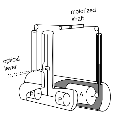
But how do we know that this prediction is even correct? Can it be verified in the laboratory? The classic laboratory test of the strength of a gravitational source is the 1797 Cavendish experiment, in which a torsion balance was used to measure the very weak gravitational attractions between metal spheres. We could test this aspect of general relativity by doing a Cavendish experiment with boxes full of photons, so that the pressure is of the same order of magnitude as the mass-energy. This is unfortunately utterly impractical, since both P and \(\rho\) for a well-lit box are ridiculously small compared to \(\rho\) for a metal ball.

Figure_8.1.1b.png" />

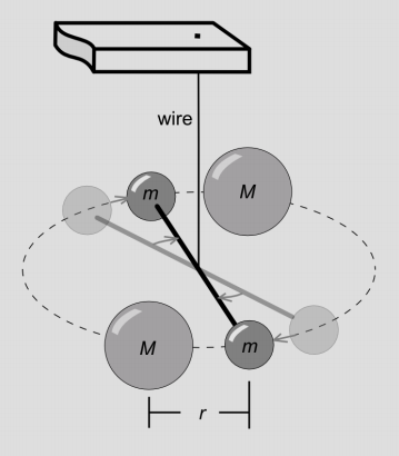
Figure \(\PageIndex{1}\) - A Cavendish balance, used to determine the gravitational constant.

However, the repulsive electromagnetic pressure inside an atomic nucleus is quite large by ordinary standards — about 10³³ Pa! To see how big this is compared to the nuclear mass density of \(\rho ∼ 10^{18}\) kg/m³, we need to take into account the factor of c² ≠ 1 in SI units, the result being that \(\frac{P}{\rho}\) is about 10⁻², which is not too small. Thus if we measure gravitational interactions of nuclei with different values of \(\frac{P}{\rho}\), we should be able to test this prediction of general relativity. This was done in a Princeton PhD-thesis experiment by Kreuzer¹ in 1966.

Before we can properly describe and interpret the Kreuzer experiment, we need to distinguish the several different types of mass that could in principle be different from one another in a theory of gravity. We’ve already encountered the distinction between inertial and gravitational mass, which Eötvös experiments show to be equivalent to about one part in 10¹². But there is also a distinction between an object’s active gravitational mass m_a, which measures its ability to create gravitational fields, and its passive gravitational mass mp, which measures the force it feels when placed in an externally generated field. For experiments using laboratoryscale material objects at nonrelativistic velocities, the Newtonian limit applies, and we can think of active gravitational mass as a scalar, with a density T^tt = \(\rho\).

To understand how this relates to pressure as a source of gravitational fields, it is helpful to consider a case where P is about the same as \(\rho\), which occurs for light. Light is inherently relativistic, so the Newtonian concept of a scalar gravitational mass breaks down, but we can still use “mass” in quotes to talk qualitatively about an electromagnetic wave’s active and passive participation in gravitational effects. Experiments show that general relativity correctly predicts the deflection of light by the sun to about one part in 10⁵ (section 6.2). This is the electromagnetic equivalent of an Eötvös experiment; it shows that general relativity predicts the right thing about the proportion between a light wave’s inertial and passive gravitational “masses.” Now suppose that general relativity was wrong, and pressure was not a source of gravitational fields. This would cause a drastic decrease in the active gravitational “mass” of an electromagnetic wave.

The Kreuzer experiment actually dealt with static electric fields inside nuclei, not electromagnetic waves, but it is still clear what we should expect in general: if pressure does not act as a gravitational source, then the ratio \(\frac{m_{a}}{m_{p}}\) should be different for different nuclei. Specifically, it should be lower for a nucleus with a higher atomic number Z, in which the electrostatic pressures are higher.

Kreuzer did a Cavendish experiment, Figure 8.1.2, using masses made of two different substances. The first substance was teflon. The second substance was a mixture of the liquids trichloroethylene and dibromoethane, with the proportions chosen so as to give a density as close as possible to that of teflon. Teflon is 76% fluorine by weight, and the liquid is 74% bromine. Fluorine has atomic number Z = 9, bromine Z = 35, and since the electromagnetic force has a long range, the pressure within a nucleus scales upward roughly like Z^1/3 (because any given proton is acted on by Z − 1 other protons, and the size of a nucleus scales like Z 1/3 , so \(P \propto \frac{Z}{(Z^{1/3})^{2}}\). The solid mass was immersed in the liquid, and the combined gravitational field of the solid and the liquid was detected by a Cavendish balance.

Figure \(\PageIndex{2}\) - A simplified diagram of Kreuzer’s modification. The moving teflon mass is submerged in a liquid with nearly the same density.

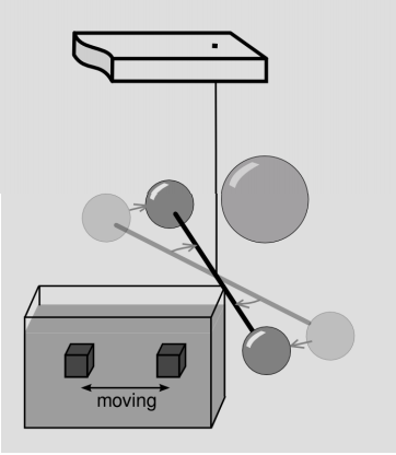
Ideally, one would formulate the liquid mixture so that its passivemass density was exactly equal to that of teflon, as determined by buoyancy. Any oscillation in the torque measured by the Cavendish balance would then indicate an inequivalence between active and passive gravitational mass.

Figure_8.1.3b.png" />

Figure \(\PageIndex{3}\) - The Kreuzer experiment. 1. There are two passive masses, P, and an active mass A consisting of a single 23-cm diameter teflon cylinder immersed in a fluid. The teflon cylinder is driven back and forth with a period of 400 s. The resulting deflection of the torsion beam is monitored by an optical lever and canceled actively by electrostatic forces from capacitor plates (not shown). The voltage required for this active cancellation is a measure of the torque exerted by A on the torsion beam. 2. Active mass as a function of temperature. 3. Passive mass as a function of temperature. In both 2 and 3, temperature is measured in units of ohms, i.e., the uncalibrated units of a thermistor that was immersed in the liquid.

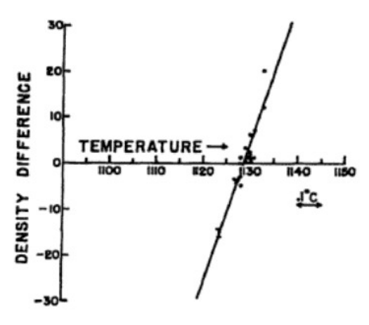
In reality, the two substances involved had different coefficients of thermal expansion, so slight variations in temperature made their passive-mass densities unequal. Kreuzer therefore measured both the buoyant force and the gravitational torque as functions of temperature. He determined that these became zero at the same temperature, to within experimental errors, which verified the equivalence of active and passive gravitational mass to within a certain precision,

\[m_{p} \propto m_{a}\]

to within 5 × 10⁻⁵.

Kreuzer intended this exeriment only as a test of m_p ∝ m_a, but it was reinterpreted in 1976 by Will² as a test of the coupling of sources to gravitational fields as predicted by general relativity and other theories of gravity. Crudely, we’ve already argued that mp ∝ ma would be substance-dependent if pressure did not couple to gravitational fields. Will actually carried out a more careful calculation, of which I present a simplified summary. Suppose that pressure does not contribute as much to gravitational fields as is claimed by general relativity; its coupling is reduced by a factor 1 − x, where x = 0 in general relativity.³ Will considers a model consisting of pointlike particles interacting through static electrical forces, and shows that for such a system,

\[m_{a} = m_{p} + \frac{1}{2} x U_{e},\]

where U_e is the electrical energy. The Kreuzer experiment then requires |x| < 6 × 10⁻², meaning that pressure does contribute to gravitational fields as predicted by general relativity, to within a precision of 6%.

Note

In Will’s notation, \(\zeta_{4}\) measures nonstandard coupling to pressure, \(\zeta_{3}\) to internal energy, and \(\zeta_{1}\) to kinetic energy. By requiring that point-particle models agree with perfect-fluid models, one obtains \((−\frac{2}{3}) \zeta_{1} = \zeta_{3} = − \zeta_{4} = x\).

One of the important ways in which Will’s calculation goes beyond my previous crude argument is that it shows that when x = 0, as it does for general relativity, the correction term \(\frac{xU_{e}}{2}\) vanishes, and m_a = m_p exactly. This is interpreted as follows. Let a bromine nucleus be referred to with a capital M, fluorine with the lowercase m. Then when a bromine nucleus and a fluorine nucleus interact gravitationally at a distance r, the Newtonian approximation applies, and the total internal force acting on the pair of nuclei taken as a whole equals \(\frac{m_{p} M_{a} − M_{p} m_{a}}{r^{2}}\) (in units where the Newtonian gravitational constant G equals 1). This vanishes only if m_pM_a − M_pm_a = 0, which is equivalent to \(\frac{m_{p}}{M_{p}} = \frac{m_{a}}{M_{a}}\). If this proportionality fails, then the system violates Newton’s third law and conservation of momentum; its center of mass will accelerate along the line connecting the two nuclei, either in the direction of M or in the direction of m, depending on the sign of x.

Thus the vanishing of the correction term \(\frac{xU_{e}}{2}\) tells us that general relativity predicts exact conservation of momentum in this interaction. This is comforting, but a little surprising on the face of it. Newtonian gravity treats active and passive massive perfectly symmetrically, so that there is a perfect guarantee of conservation of momentum. But relativity incorporates them in a completely asymmetric manner, so there is no obvious reason that we should have perfect conservation of momentum. In fact we don’t have any general guarantee of conservation of momentum, since, as discussed in section 4.5, the language of general relativity doesn’t even give us the symbols we would need in order to state a global conservation law for a vector. General relativity does, however, allow local conservation laws. We will have local conservation of mass-energy and momentum provided that the stress-energy tensor’s divergence \(\nabla_{b} T^{ab}\) vanishes.

Bartlett and van Buren⁴ used this connection to conservation of momentum in 1986 to derive a tighter limit on x. Since the moon has an asymmetrical distribution of iron and aluminum, a nonzero x would cause it to have an anomalous acceleration along a certain line. Because lunar laser ranging gives extremely accurate data on the moon’s orbit, the constraint is tightened to |x| < 1 × 10⁻⁸.

Figure \(\PageIndex{4}\) - The Apollo 11 mission left behind this mirror, which in this photo shows the reflection of the black sky. The mirror is used for lunar laser ranging measurements, which have an accuracy of about a centimeter.

These are tests of general relativity’s predictions about the gravitational fields generated by the pressure of a static electric field. In addition, there is indirect confirmation (section 8.2) that general relativity is correct when it comes to electromagnetic waves.

References

¹ Kreuzer, Phys. Rev. 169 (1968) 1007

² Will, “Active mass in relativistic gravity: Theoretical interpretation of the Kreuzer experiment,” Ap. J. 204 (1976) 234, available online at adsabs. harvard.edu. A broader review of experimental tests of general relativity is given in Will, “The Confrontation between General Relativity and Experiment,” relativity.livingreviews.org/Articles/lrr-2006-3/. The Kreuzer experiment is discussed in section 3.7.

⁴ Phys. Rev. Lett. 57 (1986) 21. The result is summarized in section 3.7 of the review by Will.