8.3: Cosmological Solutions (Part I)

We are thus led to pose two interrelated questions. First, what can empirical observations about the universe tell us about the laws of physics, such as the zero or nonzero value of the cosmological constant? Second, what can the laws of physics, combined with observation, tell us about the large-scale structure of the universe, its origin, and its fate?

Evidence for the Finite Age of the Universe

We have a variety of evidence that the universe’s existence does not stretch for an unlimited time into the past.

When astronomers view light from the deep sky that has been traveling through space for billions of years, they observe a universe that looks different from today’s. For example, quasars were common in the early universe but are uncommon today.

In the present-day universe, stars use up deuterium nuclei, but there are no known processes that could replenish their supply. We therefore expect that the abundance of deuterium in the universe should decrease over time. If the universe had existed for an infinite time, we would expect that all its deuterium would have been lost, and yet we observe that deuterium does exist in stars and in the interstellar medium.

The second law of thermodynamics predicts that any system should approach a state of thermodynamic equilibrium, and yet our universe is very far from thermal equilibrium, as evidenced by the fact that our sun is hotter than interstellar space, or by the existence of functioning heat engines such as your body or an automobile engine.

With hindsight, these observations suggest that we should not look for cosmological models that persist for an infinite time into the past.

Evidence for Expansion of the Universe

We don’t only see time-variation in locally observable quantities such as quasar abundance, deuterium abundance, and entropy. In addition, we find empirical evidence for global changes in the universe. By 1929, Edwin Hubble at Mount Wilson had determined that the universe was expanding, and historically this was the first convincing evidence that Einstein’s original goal of modeling a static cosmology had been a mistake. Einstein later referred to the cosmological constant as the “greatest blunder of my life,” and for the next 70 years it was commonly assumed that \(\Lambda\) was exactly zero.

Since we observe that the universe is expanding, the laws of thermodynamics require that it also be cooling, just as the exploding air-gas mixture in a car engine’s cylinder cools as it expands. If the universe is currently expanding and cooling, it is natural to imagine that in the past it might have been very dense and very hot. This is confirmed directly by looking up in the sky and seeing radiation from the hot early universe. In 1964, Penzias and Wilson at Bell Laboratories in New Jersey detected a mysterious background of microwave radiation using a directional horn antenna. As with many accidental discoveries in science, the important thing was to pay attention to the surprising observation rather than giving up and moving on when it confounded attempts to understand it. They pointed the antenna at New York City, but the signal didn’t increase. The radiation didn’t show a 24-hour periodicity, so it couldn’t be from a source in a certain direction in the sky. They even went so far as to sweep out the pigeon droppings inside. It was eventually established that the radiation was coming uniformly from all directions in the sky and had a black-body spectrum with a temperature of about 3 K.

Figure \(\PageIndex{1}\) - The horn antenna used by Penzias and Wilson.

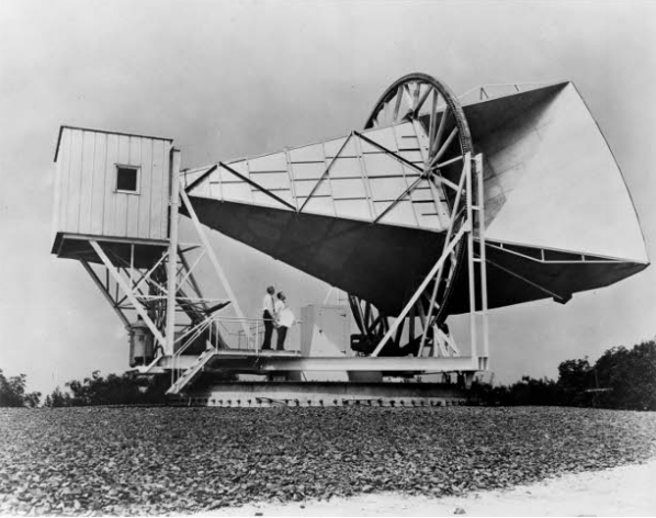
This is now interpreted as follows. At one time, the universe was hot enough to ionize matter. An ionized gas is opaque to light, since the oscillating fields of an electromagnetic wave accelerate the charged particles, depositing kinetic energy into them. Once the universe became cool enough, however, matter became electrically neutral, and the universe became transparent. Light from this time is the most long-traveling light that we can detect now. The latest data show that transparency set in when the temperature was about 3000 K. The surface we see, dating back to this time, is known as the surface of last scattering. Since then, the universe has expanded by about a factor of 1000, causing the wavelengths of photons to be stretched by the same amount due to the expansion of the underlying space. This is equivalent to a Doppler shift due to the source’s motion away from us; the two explanations are equivalent. We therefore see the 3000 K optical black-body radiation red-shifted to 3 K, in the microwave region.

It is logically possible to have a universe that is expanding but whose local properties are nevertheless static, as in the steady-state model of Fred Hoyle, in which some novel physical process spontaneously creates new hydrogen atoms, preventing the infinite dilution of matter over the universe’s history, which in this model extends infinitely far into the past. But we have already seen strong empirical evidence that the universe’s local properties (quasar abundance, etc.) are changing over time. The CMB is an even more extreme and direct example of this; the universe full of hot, dense gas that emitted the CMB is clearly nothing like today’s universe. A brief discussion of the steady-state model is given in section 8.4.

Evidence for Homogeneity and Isotropy

These observations demonstrate that the universe is not homogeneous in time, i.e., that one can observe the present conditions of the universe (such as its temperature and density), and infer what epoch of the universe’s evolution we inhabit. A different question is the Copernican one of whether the universe is homogeneous in space. Surveys of distant quasars show that the universe has very little structure at scales greater than a few times 10²⁵ m. (This can be seen on a remarkable logarithmic map constructed by Gott et al., astro.princeton.edu/universe.) This suggests that we can, to a good approximation, model the universe as being isotropic (the same in all spatial directions) and homogeneous (the same at all locations in space). (Isotropy does not follow from homogeneity. Examples of homogeneous but anisotropic cosmologies include rotating cosmologies and the Kantowsky-Sachs metric, problem 13.)

Further evidence comes from the extreme uniformity of the cosmic microwave background radiation, once one subtracts out the dipole anisotropy due to the Doppler shift arising from our galaxy’s motion relative to the CMB. When the CMB was first discovered, there was doubt about whether it was cosmological in origin (rather than, say, being associated with our galaxy), and it was expected that its isotropy would be as large as 10%. As physicists began to be convinced that it really was a relic of the early universe, interest focused on measuring this anisotropy, and a series of measurements put tighter and tighter upper bounds on it. Other than the dipole term, there are two ways in which one might naturally expect anisotropy to occur. There might have been some lumpiness in the early universe, which might have served as seeds for the condensation of galaxy clusters out of the cosmic medium. Furthermore, we might wonder whether the universe as a whole is rotating. The general-relativistic notion of rotation is very different from the Newtonian one, and in particular, it is possible to have a cosmology that is rotating without having any center of rotation (see problem 5). In fact one of the first exact solutions discovered for the Einstein field equations was the Gödel metric, which described a bizarre rotating universe with closed timelike curves, i.e., one in which causality was violated. In a rotating universe, one expects that radiation received from great cosmological distances will have a transverse Doppler shift, i.e., a shift originating from the time dilation due to the motion of the distant matter across the sky. This shift would be greatest for sources lying in the plane of rotation relative to us, and would vanish for sources lying along the axis of rotation. The CMB would therefore show variation with the form of a quadrupole term, 3 cos² \(\theta\) − 1. In 1977 a U-2 spyplane (the same type involved in the 1960 U.S.-Soviet incident) was used by Smoot et al.¹⁴ to search for anisotropies in the CMB. This experiment was the first to definitively succeed in detecting the dipole anisotropy. After subtraction of the dipole component, the CMB was found to be uniform at the level of ∼ 3 × 10⁻⁴. This provided strong support for homogeneous cosmological models, and ruled out rotation of the universe with \(\omega \gtrsim\) 10⁻²² Hz.

Note

G. F. Smoot, M. V. Gorenstein, and R. A. Muller, “Detection of Anisotropy in the Cosmic Blackbody Radiation,” Phys. Rev. Lett. 39 (1977) 898. The interpretation of the CMB measurements is somewhat model-dependent; in the early years of observational cosmology, it was not even universally accepted that the CMB had a cosmological origin. The best model-independent limit on the rotation of the universe comes from observations of the solar system, Clemence, “Astronomical Time,” Rev. Mod. Phys. 29 (1957) 2.

The FRW Cosmologies

The FRW Metric and the Standard Coordinates

Motivated by Hubble’s observation that the universe is expanding, we hypothesize the existence of solutions of the field equation in which the properties of space are homogeneous and isotropic, but the over-all scale of space is increasing as described by some scale function a(t). Because of coordinate invariance, the metric can still be written in a variety of forms. One such form is

\[ds^{2} = dt^{2} - a(t)^{2} d \ell^{2},\]

where the spatial part is

\[d \ell^{2} = f(r) dr^{2} + r^{2} d \theta^{2} + r^{2} \sin^{2} \theta d \phi^{2} \ldotp\]

To interpret the coordinates, we note that if an observer is able to determine the functions a and f for her universe, then she can always measure some scalar curvature such as the Ricci scalar or the Kretchmann invariant, and since these are proportional to a raised to some power, she can determine a and t. This shows that t is a “look-out-the-window” time, i.e., a time coordinate that we can determine by looking out the window and observing the present conditions in the universe. Because the quantity being measured directly is a scalar, the result is independent of the observer’s state of motion. (In practice, these scalar curvatures are difficult to measure directly, so we measure something else, like the sky-wide average temperature of the cosmic microwave background.) Simultaneity is supposed to be ill-defined in relativity, but the look-out-the-window time defines a notion of simultaneity that is the most naturally interesting one in this spacetime. With this particular definition of simultaneity, we can also define a preferred state of rest at any location in spacetime, which is the one in which t changes as slowly as possible relative to one’s own clock. This local rest frame, which is more easily determined in practice as the one in which the microwave background is most uniform across the sky, can also be interpreted as the one that is moving along with the Hubble flow, i.e., the average motion of the galaxies, photons, or whatever else inhabits the spacetime. The time t is interpreted as the proper time of a particle that has always been locally at rest. The spatial distance measured by L = \(\int\) a d\(\ell\) is called the proper distance. It is the distance that would be measured by a chain of rulers, each of them “at rest” in the above sense.

These coordinates are referred as the “standard” cosmological coordinates; one will also encounter other choices, such as the comoving and conformal coordinates, which are more convenient for certain purposes. Historically, the solution for the functions a and f was found by de Sitter in 1917.

The spatial metric

The unknown function f(r) has to give a 3-space metric d\(\ell^{2}\) with a constant Einstein curvature tensor. The following Maxima program computes the curvature.

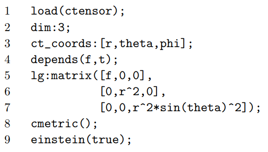
Line 2 tells Maxima that we’re working in a space with three dimensions rather than its default of four. Line 4 tells it that f is a function of time. Line 9 uses its built-in function for computing the Einstein tensor G^a_b. The result has only one nonvanishing component, \(G^{t}_{t} = \frac{1 − \frac{1}{f}}{r^{2}}\). This has to be constant, and since scaling can be absorbed in the factor a(t) in the 3+1-dimensional metric, we can just set the value of G_tt more or less arbitrarily, except for its sign. The result is f = \(\frac{1}{1 − kr^{2}}\), where k = −1, 0, or 1.

The resulting metric, called the Robertson-Walker metric, is

\[ds^{2} = dt^{2} - a^{2} \left(\dfrac{dr^{2}}{1 - kr^{2}} + r^{2} d \theta^{2} + r^{2} \sin^{2} \theta d \phi^{2} \right) \ldotp\]

The form of d\(\ell^{2}\) shows us that k can be interpreted in terms of the sign of the spatial curvature. We recognize the k = 0 metric as a flat spacetime described in spherical coordinates. To interpret the k ≠ 0 cases, we note that a circle at coordinate r has proper circumference C = 2\(\pi\)ar and proper radius R = \(a \int_{0}^{r} \sqrt{f(r')}\) dr'. For k < 0, we have f < 1 and C > 2\(\pi\)R, indicating negative spatial curvature. For k > 0 there is positive curvature.

Let’s examine the positive-curvature case more closely. Suppose we select a particular plane of simultaneity defined by t = constant and \(\phi = \frac{\pi}{2}\), and we start doing geometry in this plane. In two spatial dimensions, the Riemann tensor only has a single independent component, which can be identified with the Gaussian curvature (sec. 5.4), and when this Gaussian curvature is positive and constant, it can be interpreted as the angular defect of a triangle per unit area (sec. 5.3). Since the sum of the interior angles of a triangle can never be greater than 3\(\pi\), we have an upper limit on the area of any triangle. This happens because the positive-curvature Robertson-Walker metric represents a cosmology that is spatially finite. At a given t, it is the three-dimensional analogue of a two-sphere. On a two-sphere, if we set up polar coordinates with a given point arbitrarily chosen as the origin, then we know that the r coordinate must “wrap around” when we get to the antipodes. That is, there is a coordinate singularity there. (We know it can only be a coordinate singularity, because if it wasn’t, then the antipodes would have special physical characteristics, but the FRW model was constructed to be spatially homogeneous.) This “wrap-around” behavior is described by saying that the model is closed.

Figure \(\PageIndex{2}\) - 1. In the Euclidean plane, this triangle can be scaled by any factor while remaining similar to itself. 2. In a plane with positive curvature, geometrical figures have a maximum area and maximum linear dimensions. This triangle has almost the maximum area, because the sum of its angles is nearly 3\(\pi\). 3. In a plane with negative curvature, figures have a maximum area but no maximum linear dimensions. This triangle has almost the maximum area, because the sum of its angles is nearly zero. Its vertices, however, can still be separated from one another without limit.

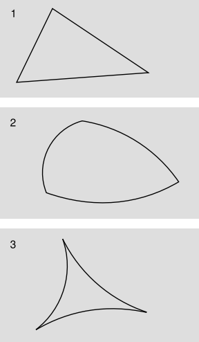
In the negative-curvature case, there is no limit on distances, Figure 8.2.2 (3). Such a universe is called open. In the case of an open universe, it is particularly easy to demonstrate a fact that bothers many students, which is that proper distances can grow at rates exceeding c. Let particles A and B both be at rest relative to the Hubble flow. The proper distance between them is then given by L = a\(\ell\), where \(\ell = \int_{A}^{B} d\ell\) is constant. Then differentiating L with respect to the look-out-the-window time t gives \(\frac{dL}{dt} = \dot{a} \ell\). In an open universe, there is no limit on the size of \(\ell\), so at any given time, we can make \(\frac{dL}{dt}\) as large as we like. This does not violate special relativity, since it is only locally that special relativity is a valid approximation to general relativity. Because GR only supplies us with frames of reference that are local, the velocity of two objects relative to one another is not even uniquely defined; our choice of \(\frac{dL}{dt}\) was just one of infinitely many possible definitions.

The distinction between closed and open universes is not just a matter of geometry, it’s a matter of topology as well. Just as a two-sphere cannot be made into a Euclidean plane without cutting or tearing, a closed universe is not topologically equivalent to an open one. The correlation between local properties (curvature) and global ones (topology) is a general theme in differential geometry. A universe that is open is open forever, and similarly for a closed one.

The Friedmann Equations

Having fixed f(r), we can now see what the field equation tells us about a(t). The next program computes the Einstein tensor for the full four-dimensional spacetime:

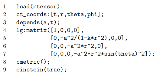
The result is

\[\begin{split} G^{t}_{t} &= 3 \left(\dfrac{\dot{a}}{a}\right)^{2} + 3ka^{-2} \\ G^{r}_{r} = G^{\theta}_{\theta} = G^{\phi}_{\phi} &= 2 \frac{\ddot{a}}{a} + \left(\dfrac{\dot{a}}{a}\right)^{2} + ka^{-2}, \end{split}\]

where dots indicate differentiation with respect to time.

Since we have G^a_b with mixed upper and lower indices, we either have to convert it into G_ab, or write out the field equations in this mixed form. The latter turns out to be simpler. In terms of mixed indices, g^a_b is always simply diag(1, 1, 1, 1). Arbitrarily singling out r = 0 for simplicity, we have g = diag(1, −a², 0, 0). The stress-energy tensor is \(T^{\mu}_{\nu}\) = diag(\(\rho\), −P, −P, −P). (See example 4 for the signs.) Substituting into G^a_b = 8\(\pi\)T^a_b + \(\Lambda\)g^a_b, we find

\[\begin{split} 3 \left(\dfrac{\dot{a}}{a}\right)^{2} + 3ka^{-2} - \Lambda &= 8 \pi \rho \\ 2 \frac{\ddot{a}}{a} + \left(\dfrac{\dot{a}}{a}\right)^{2} + ka^{-2} - \Lambda &= -8 \pi P \ldotp \end{split}\]

Rearranging a little, we have a set of differential equations known as the Friedmann equations,

\[\begin{split} \frac{\ddot{a}}{a} &= \frac{1}{3} \Lambda - \frac{4 \pi}{3} \Lambda - \frac{4 \pi}{3} (\rho + 3P) \\ \left(\dfrac{\dot{a}}{a}\right)^{2} &= \frac{1}{3} \Lambda + \frac{8 \pi}{3} \rho - ka^{-2} \ldotp \end{split}\]

The cosmology that results from a solution of these differential equations is known as the Friedmann-Robertson-Walker (FRW) or Friedmann-Lemaître-Robertson-Walker (FLRW) cosmology.

Figure \(\PageIndex{3}\) - Alexander Friedmann (1888- 1925)

The first Friedmann equation describes the rate at which cosmological expansion accelerates or decelerates. Let’s refer to it as the acceleration equation. It expresses the basic idea of the field equations, which is that non-tidal curvature (left-hand side) is caused by the matter that is present locally (right-hand side). Example 15 illustrates this in a simple case.

The second Friedmann equation tells us the magnitude of the rate of expansion or contraction. Call it the velocity equation. The quantity \(\frac{\dot{a}}{a}\), evaluated at the present cosmological time, is the Hubble constant H_o (which is constant only in the sense that at a fixed time, it is a constant of proportionality between distance and recession velocity).

To the practiced eye, it seems odd to have two dynamical laws, one predicting velocity and one acceleration. The analogous laws in freshman mechanics would be Newton’s second law, which predicts acceleration, and conservation of energy, which predicts velocity. Newton’s laws and conservation of energy are not independent, and for mechanical systems either can be derived from the other. The Friedmann equations, however, are not overdetermined or redundant. They are underdetermined, because we want to predict three unknown functions of time: a, \(\rho\), and P. Since there are only two equations, they are not sufficient to uniquely determine a solution for all three functions. The third constraint comes in the form of some type of equation of state for the matter described by \(\rho\) and P, which in simple models can often be written in the form P = w\(\rho\). For example, dust has w = 0.

Unlike a, \(\rho\), and P, the cosmological constant \(\Lambda\) is not free to vary with time; if it did, then the stress-energy tensor would have a nonvanishing divergence, which is not consistent with the Einstein field equations (see section 8.1).

Although general relativity does not provide any scalar, globally conserved measure of mass-energy that is conserved in all spacetimes, the Friedmann velocity equation can be loosely interpreted as a statement of conservation of mass-energy in an FRW spacetime. The left-hand side acts like kinetic energy. In a cosmology that expands and then recontracts in a Big Crunch, the turn-around point is defined by the time at which the right-hand side equals zero. The origin of the velocity equation is in fact the time-time part of the field equations, whose source term is the mass-energy component of the stress-energy tensor.

Example 15: Scooping out a hole

Figure \(\PageIndex{4}\)

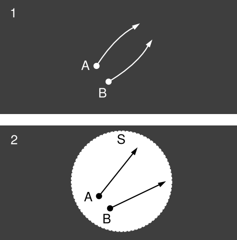
This example illustrates the connection between cosmological acceleration and local density of matter given by the Friedmann acceleration equation. Consider two cosmologies, each with \(\Lambda\) = 0. Cosmology 1 is an FRW spacetime in which all matter is in the form of nonrelativistic particles such as atoms or galaxies. 2 is identical to 1, except that all the matter has been scooped out of a small spherical region S, leaving a vacuum. (“Small” means small compared to the Hubble scale \(\frac{1}{H_{o}}\).) Within S, we introduce test particles A and B. Because an FRW spacetime is homogeneous and isotropic, cosmology 2 retains spherical symmetry about the center of S. Since \(\Lambda\) = 0, Birkhoff’s theorem applies to 2, so 2 is flat inside S. Therefore in 2, the relative acceleration a of the test particles equals zero.

Because S is small compared to cosmological distances, and because the dust is nonrelativistic, local observers can accurately attibute the difference in behavior between 1 and 2 to the Newtonian gravitational force from the dust that was present in 1 but not in 2. For convenience, let A and B both be initially at rest relative to the local dust (i.e., having \(\dot{\theta} = \dot{\phi} = 0\)). By the definition of the scale factor (i.e., by inspection of the FRW metric), the distance between them varies as const × a(t). If one of these particles is an observer, she sees a “force” acting on the other particle that causes an acceleration (a¨ /a)r, where r is the displacement between the particles.

Since a = 0 in 2, it follows that the acceleration in 1 can be calculated accurately by finding the Newtonian gravitational force due to the added dust. This results in a connection between \(\frac{\ddot{a}}{a}\), on the left-hand side of the Friedmann acceleration equation, and \(\rho\), on the right side.

For consistency, we can verify that the Newtonian gravitational force exerted by a uniform sphere, at a point on its interior, is proportional to r. This is a classic result that is easily derived from Newton’s shell theorem.