10.7: Maxwell’s Equations

Learning Objectives

• Explain Maxwell's Equations

Statement and interpretation

In this book I assume that you’ve had the usual physics background acquired in a freshman survey course, which includes an initial, probably frightening, encounter with Maxwell’s equations in integral form. In units with $c=1$, Maxwell’s equations are:

Maxwell's equation

$$\Phi_E = 4\pi kq$$

$$\Phi_B = 0$$

$$\oint \vec{E}\cdot dl = -\frac{\partial \Phi _B}{\partial t}$$

$$\oint \vec{B}\cdot dl = \frac{\partial \Phi _E}{\partial t} + 4\pi kI$$

where

$$\Phi_E = \int E\cdot da$$

and

$$\Phi_B = \int B\cdot da$$

Equations $\PageIndex{1}$ and $\PageIndex{2}$ refer to a closed surface and the charge $q$ contained inside that surface. Equation , Gauss’s law, says that charges are the sources of the electric field, while says that magnetic "charges" don’t exist. Equations $\PageIndex{3}$ and $\PageIndex{4}$ refer to a surface like a potato chip, which has an edge or boundary, and the current $I$ passing through that surface, with the line integrals in being evaluated along that boundary. The right-hand side of says that a changing magnetic field produces a curly electric field, as in a generator or a transformer. The $I$ term in says that currents create magnetic fields that curl around them. The $\partial \Phi_E/\partial t$ term, which says that changing electric fields create magnetic fields, is necessary so that the equations produce consistent results regardless of the surfaces chosen, and is also part of the apparatus responsible for the existence of electromagnetic waves, in which the changing $\vec{E}$ field produces the $\vec{B}$, and the changing $\vec{B}$ makes the $\vec{E}$.

Equations $\PageIndex{1}$ and $\PageIndex{2}$ have no time-dependence. They function as constraints on the possible field patterns. Equations $\PageIndex{3}$ and $\PageIndex{4}$ are dynamical laws that predict how an initial field pattern will evolve over time. It can be shown that if $\PageIndex{1}$ and $\PageIndex{2}$ are satisfied initially, then $\PageIndex{3}$ and $\PageIndex{4}$ ensure that they will continue to be satisfied later. Because the dynamical laws consist of two vector equations, they provide a total of $6$ constraints, which are the number needed in order to predict the behavior of the $6$ fields $E_x$, $E_y$, $E_z$, $B_x$, $B_y$, and $B_z$. <% end_sec(‘maxwell-statement’)

Experimental Support

Before Einstein’s 1905 paper on relativity, the known laws of physics were Newton’s laws and Maxwell’s equations. Experiments such as Example 4.2.3 show that Newton’s laws are only low-velocity approximations. Maxwell’s equations are low-velocity approximations; for example, in section we noted the evidence that atoms are electrically neutral, in agreement with Gauss’s law, Equation $\PageIndex{1}$, to one part in $10^{21}$, even though the electrons in atoms typically have velocities on the order of $1-10\%$ of $c$.

Incompatibility with Galilean spacetime

Maxwell’s equations are not compatible with the Galilean description of spacetime (section 1.1). If we assume that equations hold in some frame $\vec{o}$, and then apply a Galilean boost, transforming the coordinates $(t,x,y,z)$ to $(t',x',y',z')=(t,x-vt,y,z)$, we find that in frame $\vec{o}'$ the equations have a different and more complicated form that cannot be simplified so as to look like the form they had in $\vec{o}$. Rather than writing out the resulting horrible mess and verifying that it can’t be cast back into the simpler form, an easier way to prove this is to note that there are solutions to the equations in $\vec{o}$ that are not solutions after a Galilean boost into $\vec{o}'$, if we try to keep the equations in the same form. For example, if a light wave propagates in the $x$ direction at speed $c$ in $\vec{o}$, then after a boost with $v=c$, we would have a light wave in frame $\vec{o}'$ that was standing still. (This is Einstein’s thought experiment of riding alongside a light wave on a motorcycle, section 1.1.) Such a wave would violate Equation $\PageIndex{3}$, since the left-hand side would be nonzero for a surface lying in the $xy$ plane, but the time derivative on the right-hand side would be zero.

Not manifestly relativistic in their original form

Since Maxwell’s equations are not low-velocity approximations and are incompatible with Galilean relativity, we expect with the benefit of historical hindsight that they are compatible with the relativistic picture of spacetime. But when they are expressed in the form above, they have two features, either one of which seems enough to make them completely incompatible with relativity:

1. They appear to describe instantaneous action at a distance. For example, Gauss’s law, $Φ_E = 4πkq$, relates the electric field in one place (on the closed surface) to the electric charge somewhere else (inside the surface). This nonlocal structure smells wrong relativistically, for the reasons discussed in section 10.2.
2. They appear to treat time and space asymmetrically.

What’s really happening here is that Maxwell’s equations are like a version of written in crayon on a long strip of toilet paper. They are completely relativistic, but have been written in a form that hides that fact.

The problem of nonlocality, $i$, can be shown to be a non-issue because Maxwell’s equations can be reworked into a form in which they are purely local. The idea is shown in figure $\PageIndex{1}$.

Figure $\PageIndex{1}$: A magnetic field that violates $Φ_B = 0$.

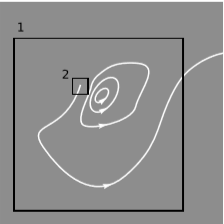
The magnetic field lines all form closed loops, except for one of them, which begins at a point in space and extends off to infinity. Drawing the large box, 1, we find that $\Phi_{B,1}$, the flux of the magnetic field through the box, is not zero, because a line leaves the box but none come in. But the same discrepancy could have been detected with the smaller box 2, or in fact with an arbitrarily small box containing the source of the field line. In other words, the equation $\Phi_B=0$ is nonlocal, but if it is to hold for any surface, then it must also hold locally, in the limit of an arbitrarily small surface. This purely law of physics can be expressed using the three-dimensional version of the divergence, introduced in section 9.1:

Of the four Maxwell’s equations, both equation $\PageIndex{1}$ and $\PageIndex{2}$ can be reexpressed in this way. This book neither presents the full machinery of vector calculus nor assumes previous knowledge of it, but a similar limiting procedure can also be applied to equations $\PageIndex{3}$ and $\PageIndex{4}$, using an operator called the curl.

The following example is one in which both problem and problem turn out not to be problems.

Example $\PageIndex{1}$: Jumping through a hoop

Figure $\PageIndex{2}$: 1. An electron jumps through a hoop. 2. An alternative surface spanning the hoop.

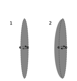
Here is an example in which the non-obvious features of Maxwell’s equations prevent the antirelativistic meltdown projected in i. In figure $\PageIndex{2}$ (1), an electron jumps back and forth through an imaginary circular hoop, across which we construct an imaginary flat surface. Every time the electron pierces the surface, it makes a momentary spike in the current $I$, which appears in:

$$\oint \vec{B}\cdot dl = \frac{\partial \Phi _E}{\partial t} + 4\pi kI$$

We might expect that this would cause the field $B$ detected on the edge of the disk to show similar spikes at the same times. But “same times” implies some notion of simultaneity, and this would be incompatible with relativity, since the t coordinate being referred to here is just one observer’s notion of time. Furthermore, it would seem that information was being transmitted instantaneously from the center of the disk to its edge, which violates relativity.

Stranger still, we can produce an apparent paradox without even appealing to relativity. Instead of the flat surface in figure $\PageIndex{2}$ (1), we can pick a dish-shaped one, figure $\PageIndex{2}$ (2), with a deep enough curve so that the electron never crosses it. The current I is always zero according to this surface, so that no field $B$ would be produced at the rim at all.

The resolution of all these difficulties lies in the term $∂Φ_E/∂t$, which we’ve ignored. With surface 1, the electron crosses the surface in time $δt$, causing a current $I = e/δt$ but also causing a change in the flux from $Φ_E ≈ 2πke$ to $Φ_E ≈ -2πke$. The result is that the right-hand side of the equation is nearly zero. With surface 2, $I = 0$ and $∂Φ_E/∂t ≈ 0$, so the right-hand side is again nearly zero.

When the approximations used above are eliminated, Maxwell’s equations do predict a nonvanishing field, which is the expected electromagnetic wave propagating away from the electron at the proper speed $c$.

Lorentz invariance

Example $\PageIndex{1}$ might seem like a "just-so story," but the apparently miraculous resolution is not a coincidence. It happens because Maxwell’s equations are in fact invariant under a Lorentz transformation, even though that isn’t obvious when they’re written in the form shown above. There are various ways of showing this:

• Einstein did it by brute force in his 1905 paper on relativity, by transforming the coordinates through a Lorentz transformation and the fields as in section 10.4.
• Maxwell’s equations are basically wave equations. (They have both wave solutions and static solutions.) We can verify that when we start with a sinusoidal plane wave in one frame, then transform into another frame, the result is again a valid sinewave solution, having been subjected to a Doppler shift (section 3.2) and aberration ( section 6.5). This requires checking that the wave is still purely transverse, but that follows easily from examining the invariants described in section 10.5. By a celebrated mathematical result called Fourier’s theorem, any well-behaved wave can be written as a sum of sine waves, and therefore any wave solution of Maxwell’s equations in one frame is also a solution in every other frame.
• Maxwell’s equations can be rewritten in terms of tensors, obeying all the grammatical rules of index gymnastics. If they can be written in this form, they are automatically Lorentz invariant.

The last approach is the most general and elegant, so we’ll provide a brief sketch of how it works. Equation $\PageIndex{1}$ has $4\pi$ times the charge on the right, while has $4\pi$ times the current. These both relate to the current four-vector $\vec{J}$, so clearly we need to combine them somehow into a single equation with $\vec{J}$ on the right. Since the local form of equation involves the three-dimensional divergence, which contains first derivatives, the left-hand side of this combined equation should have a first derivative in it. Given the grammatical rules of tensors and index gymnastics, we don’t have many possible ways to accomplish this. The only obvious thing to try is

$$\frac{\partial \mathcal{F}^{\mu\nu}}{\partial x^\nu} = 4\pi k J^\mu$$

Writing this out for $\mu$ being the time coordinate, we get a relation that equates the divergence of $\vec{E}$ to $4\pi$ times the charge density; this is the local equivalent of Equation $\PageIndex{1}$. If you’ve taken vector calculus and know about the curl operator and Stokes’ theorem, then you can verify that for $\mu$ referring to $x$, $y$, and $z$, we recover the local form of Equation $\PageIndex{4}$. The tensorial way of expressing Equation $\PageIndex{2}$ and Equation $\PageIndex{3}$ turns out to be

$$\frac{\partial \mathcal{F} ^{\mu\nu}}{\partial x^\lambda} + \frac{\partial \mathcal{F} ^{\nu\lambda}}{\partial x^\mu} + \frac{\partial \mathcal{F} ^{\lambda\mu}}{\partial x^\nu} = 0$$

Example $\PageIndex{2}$: A generator

Figure $\PageIndex{3}$: A crude, impractical generator.

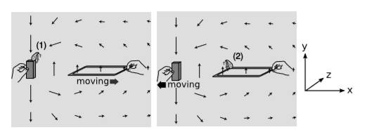
Figure $\PageIndex{3}$ shows a crude, impractical generator, depicted in two frames of reference.

Flea 1 is sitting on top of the bar magnet, which creates the magnetic field pattern shown with the arrows. To her, the bar magnet is obviously at rest, and this magnetic field pattern is static. As the square wire loop is dragged away from her and the magnet, its protons experience a force in the−$z$ direction, as determined by the Lorentz force law $\vec{F} = q\vec{v} × \vec{B}$. The electrons, which are negatively charged, feel a force in the $+z$ direction. The conduction electrons are free to move, but the protons aren’t. In the front and back sides of the loop, this force is perpendicular to the wire. In the right and left sides, however, the electrons are free to respond to the force. Since the magnetic field is weaker on the right side, current circulates around the loop.

Flea 2 is sitting on the loop, which she considers to be at rest. In her frame of reference, it’s the bar magnet that is moving. Like flea 1, she observes a current circulating around the loop, but unlike flea 1, she cannot use magnetic forces to explain this current. As far as she is concerned, the electrons were initially at rest. Magnetic forces are forces between moving charges and other moving charges, so a magnetic field can never accelerate a charged particle starting from rest. A force that accelerates a charge from rest can only be an electric force, so she is forced to conclude that there is an electric field in her region of space. This field drives electrons around and around in circles — it is a curly field. What reason can flea 2 offer for the existence of this electric field pattern? Well, she’s been noticing that the magnetic field in her region of space has been changing, possibly because that bar magnet over there has been getting farther away. She observes that a changing magnetic field creates a curly electric field. Thus the $∂Φ_B/∂t$ term in equation ( $\PageIndex{3}$) is not optional; it is required to exist if Maxwell’s equations are to be equally valid in all frames.

Einstein opens his 1905 paper on relativity¹ begins with this sentence: “It is known that Maxwell’s electrodynamics—as usually understood at the present time—when applied to moving bodies, leads to asymmetries which do not appear to be inherent in the phenomena.” He then gives essentially this example. Although the observers in frames 1 and 2 agree on all physical measurements, their explanations of the physical mechanisms, couched in the language of Maxwell’s equations in the form, are completely different. In relativistic language, flea 2’s explanation can be written in terms of equation $\PageIndex{9}$, in the case where the indices are $x$, $z$, and $t$:

$$\frac{\partial \mathcal{F} ^{xz}}{\partial t} + \frac{\partial \mathcal{F} ^{zt}}{\partial x} + \frac{\partial \mathcal{F} ^{tx}}{\partial z} = 0$$

which is the same as

$$\frac{\partial B_y}{\partial t} + \frac{\partial E_z}{\partial x} + \frac{\partial E_x}{\partial z} = 0$$

Because the first term is negative, the second term must be positive. Since equations $\PageIndex{8}$ and $\PageIndex{9}$ are written in terms of tensors, obeying the grammatical rules of index gymnastics, we are guaranteed that they give consistent predictions in all frames of reference.

Example $\PageIndex{3}$: Conservation of charge and energy-momentum

Solving equation $\PageIndex{8}$ for the current vector, we have

$$J^\mu = \frac{1}{4\pi k }\frac{\partial \mathcal{F}^{\mu\nu}}{\partial x^\nu}$$

Conservation of charge ( section 9.1) can be expressed as

$$\frac{\partial J^\mu }{\partial x^\mu} = 0$$

If we substitute the first equation into the second, we obtain

$$\frac{\partial }{\partial x^\mu} \left ( \frac{1}{4\pi k }\frac{\partial \mathcal{F}^{\mu\nu}}{\partial x^\nu} \right ) = 0$$

or

$$\frac{\partial^2 \mathcal{F}^{\mu\nu}}{\partial x^\mu \partial x^\nu} = 0$$

with a sum over both $µ$ and $ν$. But this equation is automatically satisfied because $\mathcal{F}$ is antisymmetric, so for every combination of indices $µ$ and $ν$, the term involving $\mathcal{F}^{µν}$ is canceled by one containing $\mathcal{F}^{νµ} = -\mathcal{F}^{µν}$. Thus conservation of charge does not have to be added as a supplementary condition in addition to Maxwell’s equations; it is automatically implied by Maxwell’s equations.

References

¹ “Zur Elektrodynamik bewegter K orper,” Annalen der Physik. 17 (1905) 891. Translation by Perrett and Jeffery

Contributor

• Benjamin Crowell (Fullerton College). Special Relativity is copyrighted with a CC-BY-SA license.