
9.4: Correlation Functions in the Ising Model


- Last updated
- Sep 10, 2020
- Save as PDF

( \newcommand{\kernel}{\mathrm{null}\,}\)
9.4.1 Motivation and definition
How does a spin at one site influence a spin at another site? This is not a question of thermodynamics, but it’s an interesting and useful question in statistical mechanics. The answer is given through correlation functions.
Consider an Ising model with spins si = ±1 on lattice sites i. The figure below shows part of a square lattice, although the discussion holds for any Bravais lattice in any dimension.
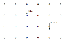
Choose a site at the center of the lattice and call it the origin, site 0. Your choice is quite arbitrary, because the lattice is infinite so any site is at the center. Now choose another site and call it site i. The product of these two spins is
s_{0} s_{i}=\left\{\begin{array}{ll}{+1} & {\text { if the spins point in the same direction }} \\ {-1} & {\text { if the spins point in opposite directions. }}\end{array}\right.
What is the average of this product over all the configurations in the ensemble? In general, this will be a difficult quantity to find, but in certain special cases we can hold reasonable expectations. For example if the system is ferromagnetic, then at low temperatures we expect that nearest neighbor spins will mostly be pointing in the same direction, whereas the opposite holds if the system is antiferromagnetic. Thus we expect that, if site i is adjacent to site 0
\left\langle s_{0} s_{i}\right\rangle \approx\left\{\begin{array}{ll}{+1} & {\text { for ferromagnetic systems at low temperatures }} \\ {-1} & {\text { for antiferromagnetic systems at low temperatures. }}\end{array}\right.
Can you think of other expectations? (High temperatures? Next-nearest-neighbors at low temperatures?) Does the average of the product ever exceed 1 in any circumstances? Let me also point out a frequently-held expectation that is not correct. One might expect that \langle s_0 s_i \rangle would vanish for sites very far apart. This is true under some circumstances, but not if an external magnetic field is applied, nor at zero field in a low-temperature ferromagnet, because in these situations all the spins in the sample (even those very far apart) tend to point in the same direction.
We have seen that the average of the product \langle s_0 s_i \rangle is not trivial. In contrast the product of the averages \langle s_0 \rangle \langle s_i \rangle is very easy, because all sites are equivalent whence \langle s_i \rangle = \langle s_0 \rangle and
\left\langle s_{0}\right\rangle\left\langle s_{i}\right\rangle=\left\langle s_{0}\right\rangle^{2}.
In fact, \langle s_0 s_i \rangle would be equal to \langle s_0 \rangle^2 if there were no correlations between spins. . . this is essentially the definition of “correlation”. This motivates the definition of the correlation function
G_{i}(T, H)=\left\langle s_{0} s_{i}\right\rangle-\left\langle s_{0}\right\rangle^{2}.
The correlation function is essentially a measure of “peer pressure”: How is the spin at site i influenced by the state of the spin at site 0? If there is a large magnetic field, for example, and if sites i and 0 are far apart, then both spins will tend to point up, but this is not because of peer pressure, it is because of “external pressure”. (For example, two children in different cities might dress the same way, not because one imitates the other, but because both listen to the same advertisements.) The term \langles_0i\rangle 2 measures external pressure, and we subtract it from \langle s_0s_i \rangle so that Gi(T, H) will measure only peer pressure and not external pressure.
This definition doesn’t say how the influence travels from site 0 to site i: If site 2 is two sites to the right of site 0, for example, then most of the influence will be due to site 0 influencing site 1 and then site 1 influencing site 2. But a little influence will travel up one site, over two sites, then down one site, and still smaller amounts will take even more circuitous routes.
Note that
\begin{aligned} \text { if } i=0 \text { then } G_{i}(T, H) &=1-\left\langle s_{0}\right\rangle^{2} \\ \text { if } i \text { is far from } 0 \text { then } & G_{i}(T, H)=0 \end{aligned}.
I have three comments to make concerning the correlation function. First, realize that the correlation function gives information about the system beyond thermodynamic information. For most of this book we have been using microscopic information to calculate a partition function and then to find macroscopic (thermodynamic) information about the system. We did not use the partition function to ask any question that involved the distance between two spins (or two atoms). The correlation function enables us to probe more deeply into statistical mechanics and ask such important microscopic questions.
Second, the correlation function is a measurable quantity. I have produced the definition through conceptual motivations1 that make it seem impossible to find except by examining individual spins. . . a conceptual nicety but experimental impossibility. But in fact the correlation function can be found experimentally through neutron scattering. This technique relies upon interference in the de Broglie waves of neutron waves scattered from nearby spins. It is not trivial: indeed two of the inventors of the technique were awarded the Nobel prize in physics for 1994. (It is also worth noting that the work of one of these two was based upon theoretical work done by Bob Weinstock in his Ph.D. thesis.) I will not have enough time to treat this interesting topic, but you should realize that what follows in this section is not mere theoretical fluff. . . it has been subjected to, and passed, the cold harsh probe of experimental test.
Third, although the definition given here applies only to Ising models on Bravais lattices, analogous definitions can be produced for other magnetic systems, for fluids, and for solids.
9.4.2 Susceptibility from the correlation function
I have emphasized above that the correlation function gives information beyond that given by thermodynamics. But the correlation function contains thermodynamic information as well. In this subsection we will prove that if the correlation function Gi(T, H) is known for all sites in the lattice, then the susceptibility, a purely thermodynamic quantity, can be found through
\chi(T, H)=N \frac{m^{2}}{k_{B} T} \sum_{i} G_{i}(T, H),
where the sum is over all sites in the lattice (including the origin).
We begin with a few reminders. The microscopic magnetization for a single configuration is
\mathcal{M}\left(s_{1}, \ldots, s_{N}\right)=m \sum_{i} s_{i}
and the macroscopic (thermodynamic) magnetization is its ensemble average
M=\langle\mathcal{M}\rangle= m N\left\langle s_{0}\right\rangle.
The Ising Hamiltonian breaks into two pieces,
\mathcal{H}=\mathcal{H}_{0}\left(s_{1}, \ldots, s_{N}\right)-m H \sum_{i} s_{i}
=\mathcal{H}_{0}\left(s_{1}, \ldots, s_{N}\right)-H \mathcal{M}\left(s_{1}, \ldots, s_{N}\right),
where \mathcal{H}_0 is independent of magnetic field. In the nearest-neighbor Ising model the field-independent part of the Hamiltonian is
\mathcal{H}_{0}\left(s_{1}, \ldots, s_{N}\right)=-J \sum_{<i, j>} s_{i} s_{j},
but we will not use this formula. . . the results of this section are true for spin-spin interactions of arbitrary complexity. Finally, the Boltzmann factor is
e^{-\beta \mathcal{H}}=e^{-\beta \mathcal{H}_{0}+\beta H \mathcal{M}}.
Now we can start the argument by examining the sum of the correlation function over all sites. In what follows, the notation \sum_{\text{s}} means the “sum over states”.
\sum_{i} G_{i}=\sum_{i}\left\langle s_{0} s_{i}\right\rangle-\left\langle s_{0}\right\rangle^{2}
=\sum_{i}\left[\frac{\sum_{\mathbf{s}} s_{0} s_{i} e^{-\beta \mathcal{H}}}{Z}-\frac{\left(\sum_{\mathbf{s}} s_{0} e^{-\beta \mathcal{H}}\right)^{2}}{Z^{2}}\right]
=\frac{\sum_{\mathbf{s}} s_{0}(\mathcal{M} / m) e^{-\beta \mathcal{H}}}{Z}-N \frac{\left(\sum_{\mathbf{s}} s_{0} e^{-\beta \mathcal{H}}\right)^{2}}{Z^{2}}
=\frac{Z \sum_{\mathrm{S}} s_{0}(\mathcal{M} / m) e^{-\beta \mathcal{H}}-N \sum_{\mathrm{S}} s_{0} e^{-\beta \mathcal{H}} \sum_{\mathrm{S}} s_{0} e^{-\beta \mathcal{N}}}{Z^{2}}
Look at this last equation carefully. What do you see? The quotient rule! Do you remember our slick trick for finding dispersions? The \mathcal{M} appearing in the leftmost summand can be gotten there by taking a derivative of equation (9.35) with respect to H:
\frac{\partial e^{-\beta \mathcal{H}}}{\partial H}=\beta \mathcal{M} e^{-\beta \mathcal{H}}.
Watch carefully:
\frac{\partial}{\partial H}\left(\frac{\sum_{\mathbf{S}} s_{0} e^{-\beta \mathcal{H}}}{Z}\right)=\frac{Z \sum_{\mathbf{S}} s_{0} \beta \mathcal{M} e^{-\beta \mathcal{H}}-\sum_{\mathbf{S}} \beta \mathcal{M} e^{-\beta \mathcal{H}} \sum_{\mathbf{S}} s_{0} e^{-\beta \mathcal{H}}}{Z^{2}}
=\beta\left[\frac{Z \sum_{\mathrm{S}} s_{0} \mathcal{M} e^{-\beta \mathcal{H}}-m N \sum_{\mathrm{S}} s_{0} e^{-\beta \mathcal{H}} \sum_{\mathrm{S}} s_{0} e^{-\beta \mathcal{H}}}{Z^{2}}\right]
But the quantity in square brackets is nothing more than m times equation (9.39),
\frac{\partial}{\partial H}\left(\frac{\sum_{\mathbf{s}} s_{0} e^{-\beta \mathcal{H}}}{Z}\right)=\beta m \sum_{i} G_{i}
But we also know that
\frac{\partial}{\partial H}\left(\frac{\sum_{s} s_{0} e^{-\beta \mathcal{H}}}{Z}\right)=\frac{\partial\left\langle s_{0}\right\rangle}{\partial H}=\frac{\partial M / m N}{\partial H}=\frac{1}{m N} \chi
whence, finally
\chi(T, H)=N \frac{m^{2}}{k_{B} T} \sum_{i} G_{i}(T, H).
Whew!
Now we can stop running and do our cool-down stretches. Does the above equation, procured at such expense, make sense? The left hand side is extensive. The right hand side has a factor of N and also sum over all sites, and usually a sum over all sites is extensive. So at first glance the left hand side scales linearly with N while the right hand side scales with N2, a sure sign of error! In fact, there is no error. The correlation function Gi vanishes except for sites very close to the origin. (“Distant sites are uncorrelated”, see equation (9.28).) Thus the sum over all sites above has a summand that vanishes for most sites, and it is intensive rather than extensive.
9.4.3 All of thermodynamics from the susceptibility
The previous subsection shows us how to find one thermodynamic quantity, χ(T, H) at some particular values for temperature and field, by knowing the correlation function Gi(T, H) for all sites i, at those same fixed values for temperature and field. In this subsection we will find how to calculate any thermodynamic quantity at all, at any value of T and H at all, by knowing χ(T, H) for all values of T and H. Thus knowing the correlation Gi(T, H) as a function of all its arguments—i, T, and H—enables us to find any thermodynamic quantity at all.
To find any thermodynamic quantity it suffices to find the free energy F(T, H), so the claim above reduces to saying that we can find F(T, H) given χ(T, H). Now we can find χ(T, H) from F(T, H) by simple differentiation, but going backwards requires some very careful integration. We will do so by looking at the difference between quantities for the Ising model and for the ideal paramagnet.
Remember that the thermodynamic state of an Ising magnet is specified by the two variables T and H, as indicated in the figure.
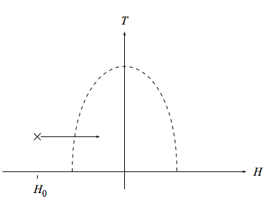
Over much of this diagram, namely the part outside the wavy line, the Ising magnet behaves very much as an ideal paramagnet does, because the typical thermal energy kBT or the typical magnetic energy m|H| overwhelms the typical spin-spin interaction energy |J|. Thus outside of the dashed line (e.g. at the ×) the Ising thermodynamic quantities are well-approximated by the paramagnetic thermodynamic quantities
\chi_{P}(T, H)=\frac{\partial M}{\partial H} )_{T}=N \frac{m^{2}}{k_{B} T} \operatorname{sech}^{2} \frac{m H}{k_{B} T}
M_{P}(T, H)=-\frac{\partial F}{\partial H} )_{T}=m N \tanh ^{2} \frac{m H}{k_{B} T}
F_{P}(T, H)=-k_{B} T N \ln \left(2 \cosh \frac{m H}{k_{B} T}\right),
and this approximation becomes better and better as T → ∞ or H → ±∞.
The difference between the susceptibility for our Ising model and for the ideal paramagnet is
\chi(T, H)-\chi_{P}(T, H)=\frac{\partial\left(M-M_{P}\right)}{\partial H} )_{T}.
Integrate this equation along the path indicated in the figure to find
\int_{H_{0}}^{H} d H^{\prime}\left[\chi\left(T, H^{\prime}\right)-\chi_{P}\left(T, H^{\prime}\right)\right]=\int_{H_{0}}^{H} d H^{\prime} \frac{\partial\left(M-M_{P}\right)}{\partial H^{\prime}} )_{T}
=\left.\left(M-M_{P}\right)\right|_{T, H}-\left.\left(M-M_{P}\right)\right|_{T, H_{0}}.
Then take the limit H0 → −∞ so that M(T, H0) → MP(T, H0) and
M(T, H)=M_{P}(T, H)+\int_{-\infty}^{H} d H^{\prime}\left[\chi\left(T, H^{\prime}\right)-\chi_{P}\left(T, H^{\prime}\right)\right],
where, remember, MP(T, H) and χP(T, H) are known functions.
We don’t have to stop here. We can consider the difference
M(T, H)-M_{P}(T, H)=-\frac{\partial\left(F-F_{P}\right)}{\partial H} )_{T}
and then perform exactly the same manipulations that we performed above to find
F(T, H)=F_{P}(T, H)-\int_{-\infty}^{H} d H^{\prime}\left[M\left(T, H^{\prime}\right)-M_{P}\left(T, H^{\prime}\right)\right].
Then we can combine equations (9.55) and (9.53) to obtain
F(T, H)=F_{P}(T, H)-\int_{-\infty}^{H} d H^{\prime} \int_{-\infty}^{H^{\prime}} d H^{\prime \prime}\left[\chi\left(T, H^{\prime \prime}\right)-\chi_{P}\left(T, H^{\prime \prime}\right)\right].
Using the known results for FP(T, H) and χP (T, H), as well as the correlation-susceptibility relation (9.46), this becomes
F(T, H)=-k_{B} T N \ln \left(2 \cosh \frac{m H}{k_{B} T}\right)-N \frac{m^{2}}{k_{B} T} \int_{-\infty}^{H} d H^{\prime} \int_{-\infty}^{H^{\prime}} d H^{\prime \prime}\left(\sum_{i} G_{i}\left(T, H^{\prime \prime}\right)-\operatorname{sech}^{2} \frac{m H^{\prime \prime}}{k_{B} T}\right).
Let me stress how remarkable this result is. You would think that to find the thermodynamic energy E(T, H) of the Ising model you would need to know the spin-spin coupling constant J. But you don’t: You can find E(T, H) without knowing J, indeed without knowing the exact form of the spin-spin interaction Hamiltonian at all, if you do know the purely geometrical information contained within the correlation function.2 This is one of the most amazing and useful facts in all of physics.
9.4.4 Parallel results for fluids
I cannot resist telling you how the results of this section change when applied to fluid rather than magnetic systems. In that case the correlation function g2(r; T, V, N) depends upon the position r rather than the site index i. Just as the sum of Gi over all sites is related to the susceptibility χ, so the integral of g2(r) over all space is related to the compressibility κT. And just as the susceptibility can be integrated twice (carefully, through comparison to the ideal paramagnet) to give the magnetic free energy F(T, H), so the compressibility can be integrated twice (carefully, through comparison to the ideal gas) to give the fluid free energy F(T, V, N). And just as the magnetic thermodynamic quantities can be found from the correlation function without knowing the details of the spin-spin interaction Hamiltonian, so the fluid thermodynamic quantities can be found from the correlation function without knowing the details of the particle interaction forces. A question for you: How is it possible to get all this information knowing only the correlation function in space rather than the correlation function in phase space? In other words, why don’t you need information about the velocities?
I should put in some references to experimental tests and to say who thought this up. Are these available in Joel’s review article?
1Namely, by asking “Wouldn’t it be nice to know how one spin is influenced by its neighbors?”
2This does not mean that the thermodynamic energy is independent of the spin-spin Hamiltonian, because the Hamiltonian influences the correlation function.