3.4: Absolute Temperature and Entropy
- Page ID
- 32021

Another consequence of the second law is the existence of an absolute temperature. Although we have used the notion of absolute temperature, it was not proven. Now we can show this just from the laws of thermodynamics.
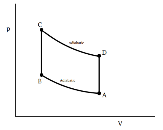
We have already seen that the efficiency of a Carnot cycle is given by
\[η = 1 − \frac{Q_2}{Q_3}\]
where \(Q_3\) is the amount of heat taken from the hotter reservoir and \(Q_2\) is the amount given up to the colder reservoir. The efficiency is independent of the material and is purely a function of the lower and upper temperatures. The system under consideration can be taken to be in thermal contact with the reservoirs, which may be considered very large. There is no exchange of particles or any other physical quantity between the reservoirs and the system, so no parameter other than the temperature can play a role in this. Let \(θ\) denote the empirically defined temperature, with \(\theta_3\) and \(θ_2\) corresponding to the reservoirs between which the engine is operating. We may thus write
\[\frac{Q_2}{Q_3} = f(θ_2, θ_3)\]
for some function \(f\) of the temperatures. Now consider another Carnot engine operating between \(θ_2\) and \(θ_1\), with corresponding Q’s, so that we have
\[\frac{Q_1}{Q_2} = f(θ_1, θ_2)\]
Now we can couple the two engines and run it together as a single engine, operating between \(θ_3\) and \(θ_1\), with
\[\frac{Q_1}{Q_3} = f(θ_1, θ_3)\]
Evidently
\[\frac{Q_2}{Q_3} \;\frac{Q_1}{Q_2} = \frac{Q_1}{Q_3}\]
so that we get the relation
\[f(θ_1, θ_2)\; f(θ_2, θ_3) = f(θ_1, θ_3)\]
This requires that the function \(f\) must be of the form
\[f(θ_1, θ_2) = \frac{f(θ_1)}{f(θ_2)}\]
for some function \(f(θ)\). Thus there must exist some function of the empirical temperature which can be defined independently of the material. This temperature is called the absolute temperature. Notice that since \(Q_1 < Q_2\), we have \(|f(θ_1)| < |f(θ_2)|\) if \(θ_1 < θ_2\). Thus \(|f|\) should be an increasing function of the empirical temperature. Further, we cannot have \(f(θ_1) = 0\) for some temperature \(θ_1\). This would require \(Q_1 = 0\). The corresponding engine would take some heat \(Q_2\) from the hotter reservoir and convert it entirely to work, contradicting the Kelvin statement. This means that we must take f to be either always positive or always negative, for all \(θ\). Conventionally we take this to be positive. The specific form of the function determines the scale of temperature. The simplest is to take a linear function of the empirical temperatures (as defined by conventional thermometers). Today, we take this to be
\[f(θ) ≡ T = \text{Temperature in Celsius} + 273.16\]
The unit of absolute temperature is the kelvin.
Once the notion of absolute temperature has been defined, we can simplify the formula for the efficiency of the Carnot engine as
\[η = 1 − \frac{T_L}{T_H}\]
Also, we have \(\frac{Q1}{Q2} = \frac{T1}{T2}\), which we may rewrite as \(\frac{Q1}{T1} = \frac{Q2}{T2}\). Since Q2 is the heat absorbed and Q1 is the heat released into the reservoir, we can assign ± signs to the Q’s, + for intake and − for release of heat, and write this equation as
\[\frac{Q_1}{T_1} + \frac{Q_2}{T_2} = 0\]
In other words, if we sum over various steps (denoted by the index i) of the cycle, with appropriate algebraic signs,
\[\sum_{cycle} \frac{Q_i}{T_i} = 0 \label{3.4.11} \]
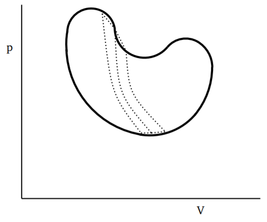
If we consider any closed and reversible cycle, as shown in Fig. 3.4.1, we can divide it into small cycles, each of which is a Carnot cycle. A few of these smaller cycles are shown by dotted lines, say with the long dotted lines being adiabatics and the short dotted lines being isothermals. By taking finer and finer such divisions, the error in approximating the cycle by a series of closed Carnot cycles will go to zero as the number of Carnot cycles goes to infinity. Since along the adiabatics, the change in \(Q\) is zero, we can use the result from Equation \ref{3.4.11} above to write
\[\oint_{cycle} \frac{dQ}{T}= 0 \label{3.4.12}\]
where we denote the heat absorbed or given up during each infinitesimal step as \(dQ\). The statement in Equation \ref{3.4.12} is due to Clausius. The important thing is that this applies to any closed curve in the space of thermodynamic variables, provided the process is reversible.
This equation has another very important consequence. If the integral of a differential around any closed curve is zero, then we can write the differential as the derivative of some function. Thus there must exist a function \(S(p, V )\) such that
\[\frac{dQ}{T} = dS,\;\;\; or\; dQ = TdS\]
This function \(S\) is called entropy. It is a function of state, given in terms of the thermodynamic variables.
Clausius’ Inequality
Clausius’ discovery of entropy is one of most important advances in the physics of material systems. For a reversible process, we have the result,
\[\oint_{cycle} \frac{dQ}{T}= \oint_{cycle} dS = 0\]
as we have already seen. There is a further refinement we can make by considering irreversible processes. There are many processes such as diffusion which are not reversible. For such a process, we cannot write \(dQ = T dS\). Nevertheless, since entropy is a function of the state of the system, we can still define entropy for each state. For an irreversible process, the heat transferred to a system is less than \(T dS\) where \(dS\) is the entropy change produced by the irreversible process. This is easily seen from the second law. For assume that a certain amount of heat \(dQ_{irr}\) is absorbed by the system in the irreversible process. Consider then a combined process where the system changes from state A to state B in an irreversible manner and then we restore state A by a reversible process. For the latter step, \(dQ_{rev} = T dS\). The combination thus absorbs an amount of heat equal to \(dQ_{irr} −T dS\) with no change of state. If this is positive, this must be entirely converted to work. However, that would violate the second law. Hence we should have
\[dQ_{irr} −T dS < 0\]
If we have a cyclic process, \(\oint dS = 0\) since \(S\) is a state function, and hence
\[\oint \frac{dQ}{T} ≤ 0\]
with equality holding for a reversible process. This is known as Clausius’ inequality.
For a system in thermal isolation, \(dQ = 0\), and the condition \(dQ_{irr} < T dS\) becomes
\[dS > 0\]
In other words, the entropy of a system left to itself can only increase, equilibrium being achieved when the entropy (for the specified values of internal energy, number of particles, etc.) is a maximum.
The second law has been used to define entropy. But once we have introduced the notion of entropy, the second law is equivalent to the statement that entropy tends to increase. For any process, we can say that
\[\frac{dS}{T} ≥ 0\]
We can actually see that this is equivalent to the Kelvin statement of the second law as follows. Consider a system which takes up heat \(∆Q\) at temperature \(T\). For the system (labeled 1) together with the heat source (labeled 2), we have \(∆S_1 + ∆S_2 ≥ 0\). But the source is losing heat at temperature \(T\) and if this is reversible, \(∆S_2 = −\frac{∆Q}{T}\). Further if there is no other change in the system, \(∆S_1 = 0\) and \(∆U_1 = 0\). Thus
\[∆S_1 + ∆S_2 ≥ 0 \Rightarrow − \frac{∆Q}{T} ≥ 0 \Rightarrow ∆Q ≤ 0\]
Since \(∆U_1 = 0, ∆Q = ∆W\) and this equation implies that the work done by the system cannot be positive, if we have \(\frac{dS}{dt} ≥ 0\). Thus, we have arrived at the Kelvin statement that a system cannot absorb heat from a source and convert it entirely to work without any other change. We may thus restate the second law in the form:
Proposition 4
Second Law of Thermodynamics: The entropy of a system left to itself will tend to increase to a maximum value compatible with the specified values of internal energy, particle number, etc.
Nature of Heat Flow
We can easily see that heat by itself flows from a hotter body to a cooler body. This may seem obvious, but is a crucial result of the second law. In some ways, the second law is the formalization of such statements which are “obvious" from our experience.
Consider two bodies at temperatures \(T_1\) and \(T_2\), thermally isolated from the rest of the universe but in mutual thermal contact. The second law tells us that \(dS ≥ 0\). This means that
\[\frac{dQ_1}{T1} + \frac{dQ_2}{T2}≥ 0\]
Because the bodies are isolated from the rest of the world, \(dQ_1 + dQ_2 = 0\), so that we can write the condition above as
\[(\frac{1}{T_1} − \frac{1}{T_2}) dQ_1 ≥ 0\]
If \(T_1 > T_2\), we must have \(dQ_1 < 0\) and if \(T_1 < T_2, dQ_1 > 0\). Either way, heat flows from the hotter body to the colder body.