2.6: Two important applications

The results of the previous section, especially Equation (\(2.5.7\)), have innumerable applications in physics and related disciplines, but here I have time for a brief discussion of only two of them.

Blackbody radiation

Let us consider a free-space volume \(V\) limited by non-absorbing (i.e. ideally reflecting) walls. Electrodynamics tells us⁴⁴ that the electromagnetic field in such a “cavity” may be represented as a sum of “modes” with the time evolution similar to that of the usual harmonic oscillator. If the volume \(V\) is large enough,⁴⁵ the number of these modes within a small range \(dk\) of the wavevector magnitude \(k\) is

\[dN = \frac{gV}{(2\pi )^3} d^3k = \frac{gV}{(2\pi)^3} 4 \pi k^2 dk, \label{82}\]

where for electromagnetic waves, the degeneracy factor \(g\) is equal to 2, due to their two different independent (e.g., linear) polarizations of waves with the same wave vector \(k\). With the linear, isotropic dispersion relation for waves in vacuum, \(k = \omega /c\), Equation (\ref{82}) yields

\[dN = \frac{2V}{(2\pi )^3} 4\pi \frac{\omega^2 d \omega}{c^3} \equiv V \frac{\omega^2}{\pi^2 c^3} d \omega \label{83}\]

On the other hand, quantum mechanics says⁴⁶ that the energy of such a “field oscillator” is quantized per Equation (\(2.2.20\)), so that at thermal equilibrium its average energy is described by Equation (\(2.5.7\)). Plugging that result into Equation (\ref{83}), we see that the spectral density of the electromagnetic field’s energy, per unit volume, is

Planck's radiation law:

\[\boxed{u(\omega) \equiv \frac{E}{V} \frac{dN}{d \omega} = \frac{\hbar \omega^3}{\pi^2 c^3} \frac{1}{e^{\hbar \omega / T} - 1} . } \label{84}\]

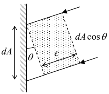
This is the famous Planck’s blackbody radiation law.⁴⁷ To understand why its common name mentions radiation, let us consider a small planar part, of area \(dA\), of a surface that completely absorbs electromagnetic waves incident from any direction. (Such “perfect black body” approximation may be closely approached using special experimental structures, especially in limited frequency intervals.) Figure \(\PageIndex{1}\) shows that if the arriving wave was planar, with the incidence angle \(\theta \), then the power \(d\mathscr{P}_{\theta} (\omega )\) absorbed by the surface of small area \(dA\), within a small frequency interval \(d\omega \), i.e. the energy incident at that area in unit time, would be equal to the radiation energy within the same frequency interval, contained inside an imaginary cylinder (shaded in Figure \(\PageIndex{1}\)) of height \(c\), base area \(dA \cos\theta \), and hence volume \(dV = c dA \cos\theta \):

\[ d\mathscr{P}_{\theta} (\omega ) = u(\omega )d\omega dV = u(\omega )d\omega c dA \cos\theta . \label{85}\]

Figure \(\PageIndex{1}\): Calculating the relation
between \(d\mathscr{P} (\omega )\) and \(u(\omega )d\omega \).

Since the thermally-induced field is isotropic, i.e. propagates equally in all directions, this result should be averaged over all solid angles within the polar angle interval \(0 \leq \theta \leq \pi /2\):

\[\frac{d \mathscr{P} ( \omega)}{dA d \omega} = \frac{1}{4\pi} \int \frac{d \mathscr{P} ( \omega)}{dA d \omega} d \Omega = cu (\omega ) \frac{1}{4\pi} \int^{\pi/2}_{0} \sin \theta d \theta \int^{2\pi }_{0} d \varphi \cos \theta = \frac{c}{4} u (\omega ). \label{86}\]

Hence the Planck’s expression (\ref{84}), multiplied by \(c/4\), gives the power absorbed by such a “blackbody” surface. But at thermal equilibrium, this absorption has to be exactly balanced by the surface’s own radiation, due to its non-zero temperature \(T\).

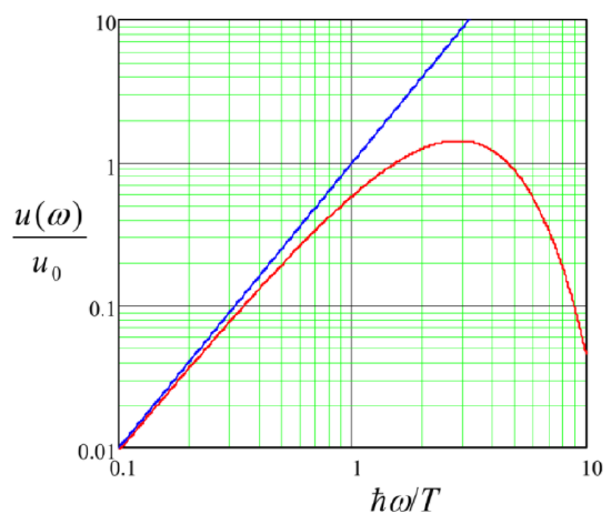
I hope the reader is familiar with the main features of the Planck law (\ref{84}), including its general shape (Figure \(\PageIndex{2}\)), with the low-frequency asymptote \(u(\omega ) \propto \omega^2\) (due to its historic significance bearing the special name of the Rayleigh-Jeans law), the exponential drop at high frequencies (the Wien law), and the resulting maximum of the function \(u(\omega )\), reached at the frequency \(\omega_{max}\) with

\[\hbar \omega_{max} \approx 2.82 T, \label{87}\]

i.e. at the wavelength \(\lambda_{max} = 2\pi /k_{max} = 2 \pi c/\omega_{max} \approx 2.22 c\hbar /T\).

Figure \(\PageIndex{2}\): The frequency dependence of the blackbody radiation density, normalized by \(u_0 \equiv T^3/\pi^2\hbar^2c^3\), according to the Planck law (red line) and the Rayleigh-Jeans law (blue line).

Still, I cannot help mentioning a few important particular values: one corresponding to the visible light (\(\lambda_{max} \sim 500\) nm) for the Sun’s effective surface temperature \(T_K \approx 6,000\) K, and another one corresponding to the mid-infrared range (\(\lambda_{max} \sim 10 \) \(\mu\)m) for the Earth’s surface temperature \(T_K \approx 300\) K. The balance of these two radiations, absorbed and emitted by the Earth, determines its surface temperature and hence has the key importance for all life on our planet. This is why it is at the front and center of the current climate change discussions. As one more example, the cosmic microwave background (CMB) radiation, closely following the Planck law with \(T_K = 2.725\) K (and hence having the maximum density at \(\lambda_{max} \approx 1.9\) mm), and in particular its (very small) anisotropy, is a major source of data for modern cosmology.

Now let us calculate the total energy \(E\) of the blackbody radiation inside some volume \(V\). It may be found from Equation (\ref{84}) by its integration over all frequencies: ^48,49

\[ E = V \int^{\infty}_0 u (\omega ) d \omega = V \int^{\infty}_0 \frac{\hbar \omega^3}{\pi^2 c^3} \frac{d\omega}{e^{\hbar \omega /T} - 1} = \frac{VT^4}{\pi^2 \hbar^3 c^3} \int^{\infty}_0 \frac{\xi^3 d \xi}{e^{\xi} -1 } = V \frac{\pi^2}{15 \hbar^3 c^3} T^4. \label{88}\]

Stefan law:

\[\boxed{ \frac{d\mathscr{P}}{dA} = \frac{\pi^2}{60\hbar^3 c^2} T^4 \equiv \sigma T^4_K , } \label{89a}\]

Stefan-Boltzmann constant:

\[\boxed{\sigma \equiv \frac{\pi^2}{60 \hbar^3 c^2} k^4_B \approx 5.67 \times 10^{-8} \frac{W}{m^2 K^4}. } \label{89b}\]

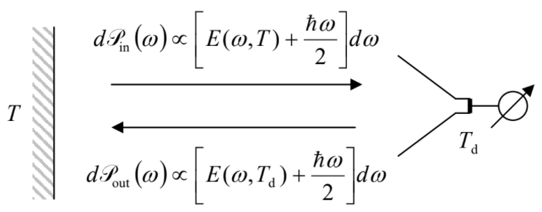
By this point, the thoughtful reader should have an important concern ready: Equation (\ref{84}) and hence Equation (\ref{88}) are based on Equation (\(2.5.7\)) for the average energy of each oscillator, referred to its ground-state energy \(\hbar \omega /2\). However, the radiation power should not depend on the energy origin; why have not we included the ground energy of each oscillator into the integration (\ref{88}), as we have done in Equation (\(2.5.15\))? The answer is that usual radiation detectors only measure the difference between the power \(\mathscr{P}_{in}\) of the incident radiation (say, that of a blackbody surface with temperature \(T\)) and their own back-radiation power \(\mathscr{P}_{out}\), corresponding to some effective temperature \(T_d\) of the detector – see Figure \(\PageIndex{3}\). But however low \(T_d\) is, the temperature-independent contribution \(\hbar \omega /2\) of the ground-state energy to the back radiation is always there. Hence, the term \(\hbar \omega /2\) drops out from the balance, and cannot be detected – at least in this simple way. This is the reason why we had the right to ignore this contribution in Equation (\ref{88}) – very fortunately, because it would lead to the integral’s divergence at its upper limit. However, let me repeat that the ground-state energy of the electromagnetic field oscillators is physically real – and important – see Sec. 5.5 below.

Figure \(\PageIndex{3}\): The power balance at the electromagnetic radiation power measurement.

One more interesting result may be deduced from the free energy \(F\) of the electromagnetic radiation, which may be calculated by integration of Equation (\(2.5.8\)) over all the modes, with the appropriate weight (\ref{83}):

\[F=\sum_{\omega} T \ln \left(1-e^{-\hbar \omega / T}\right) \rightarrow \int_{0}^{\infty} T \ln \left(1-e^{-\hbar \omega / T}\right) \frac{d N}{d \omega} d \omega=\int_{0}^{\infty} T \ln \left(1-e^{-\hbar \omega / T}\right)\left(V \frac{\omega^{2}}{\pi^{2} c^{3}}\right) d \omega. \label{90}\]

Representing \(\omega^2d\omega\) as \(d(\omega^3)/3\), we can readily work out this integral by parts, reducing it to a table integral similar to that in Equation (\ref{88}), and getting a surprisingly simple result:

\[F = -V \frac{\pi^2}{45 \hbar^3 c^3} T^4 \equiv - \frac{E}{3}. \label{91}\]

\[P = - \left( \frac{\partial F}{\partial V} \right)_T = \frac{ \pi^2}{45 \hbar^3 c^3} T^4 = \frac{E}{3V}. \label{92a}\]

Rewritten in the form,

Photon gas: \(\mathbf{PV}\) vs. \(\mathbf{E}\)

\[\boxed{ PV = \frac{E}{3},} \label{92b}\]

Finally, let me note that Equation (\ref{92a} - \ref{92b}) allows for the following interesting interpretation. The last of Eqs. (\(1.5.11\)), being applied to Equation (\ref{92a} - \ref{92b}), shows that in this particular case the grand thermodynamic potential \(\Omega\) equals \((–E/3)\), so that according to Equation (\ref{91}), it is equal to \(F\). But according to the definition of \(\Omega \), i.e. the first of Eqs. (\(1.5.11\)), this means that the chemical potential of the electromagnetic field excitations (photons) vanishes:

\[\mu = \frac{F - \Omega}{N} = 0. \label{93}\]

In Sec. 8 below, we will see that the same result follows from the comparison of Equation (\(2.5.7\)) and the general Bose-Einstein distribution for arbitrary bosons. So, from the statistical point of view, photons may be considered as bosons with zero chemical potential.

(ii) Specific heat of solids. The heat capacity of solids is readily measurable, and in the early 1900s, its experimentally observed temperature dependence served as an important test for the then-emerging quantum theories. However, the theoretical calculation of \(C_V\) is not simple⁵³ – even for insulators, whose specific heat at realistic temperatures is due to thermally-induced vibrations of their crystal lattice alone.⁵⁴ Indeed, at relatively low frequencies, a solid may be treated as an elastic continuum. Such a continuum supports three different modes of mechanical waves with the same frequency \(\omega \), that all obey linear dispersion laws, \(\omega = vk\), but the velocity \(v = v_l\) for one of these modes (the longitudinal sound) is higher than that \((v_t)\) of two other modes (the transverse sound).⁵⁵ At such frequencies, the wave mode density may be described by an evident generalization of Equation (\ref{83}):

\[dN = V \frac{1}{(2\pi)^3} \left( \frac{1}{v^3_l} + \frac{2}{v^3_t} \right) 4 \pi \omega^2 d \omega. \label{94a}\]

For what follows, it is convenient to rewrite this relation in a form similar to Equation (\ref{83}):

\[dN = \frac{3V}{(2\pi )^3} 4\pi \frac{\omega^2 d\omega}{v^3}, \quad \text{ with } v \equiv \left[ \frac{1}{3} \left( \frac{1}{v^3_l} + \frac{2}{v^3_t} \right) \right]^{-1/3}. \label{94b}\]

However, the basic wave theory shows⁵⁶ that as the frequency \(\omega\) of a sound wave in a periodic structure is increased so that its half-wavelength \(\pi /k\) approaches the crystal period \(d\), the dispersion law \(\omega (k)\) becomes nonlinear before the frequency reaches its maximum at \(k = \pi /d\). To make things even more complex, 3D crystals are generally anisotropic, so that the dispersion law is different in different directions of the wave propagation. As a result, the exact statistics of thermally excited sound waves, and hence the heat capacity of crystals, is rather complex and specific for each particular crystal type.

In 1912, P. Debye suggested an approximate theory of the specific heat’s temperature dependence, which is in a surprisingly good agreement with experiment for many insulators, including polycrystalline and amorphous materials. In his model, the linear (acoustic) dispersion law \(\omega = vk\), with the effective sound velocity \(v\) defined by the second of Eqs. (\ref{94b}), is assumed to be exact all the way up to some cutoff frequency \(\omega_D\), the same for all three wave modes. This Debye frequency may be defined by the requirement that the total number of acoustic modes, calculated within this model from Equation (\ref{94b}),

\[N = V \frac{1}{(2\pi )^3} \frac{3}{v^3} \int^{\omega_D}_0 4 \pi \omega^2 d \omega = \frac{V \omega^3_D}{2\pi^2 v^3}, \label{95}\]

is equal to the universal number \(N = 3nV\) of the degrees of freedom (and hence of independent oscillation modes) in a 3D system of \(nV\) elastically coupled particles, where \(n\) is the atomic density of the crystal, i.e. the number of atoms per unit volume.⁵⁷ For this model, Equation (\(2.5.7\)) immediately yields the following expression for the average energy and specific heat (in thermal equilibrium at temperature \(T \)):

\[E = V \frac{1}{(2\pi )^3} \frac{3}{v^3} \int^{\omega_D}_0 \frac{\hbar \omega}{e^{\hbar \omega /T}-1} 4 \pi \omega^2 d \omega \equiv 3 n VT D (x)_{x=T_D/T}, \label{96}\]

Debye law:

\[\boxed{c_V \equiv \frac{C_V}{nV} = \frac{1}{nV} \left( \frac{\partial E}{\partial T} \right)_V = 3 \left[ D(x) -x \frac{dD(x)}{dx} \right]_{x=T_D/T} , } \label{97}\]

where \(T_D \equiv \hbar \omega_D\) is called the Debye temperature,⁵⁸ and

\[D(x) \equiv \frac{3}{x^{3}} \int_{0}^{x} \frac{\xi^{3} d \xi}{e^{\xi}-1} \rightarrow \begin{cases}1, & \text { for } x \rightarrow 0 , \\ \pi^{4} / 5 x^{3}, & \text { for } x \rightarrow \infty, \end{cases} \label{98}\]

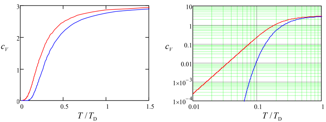
is the Debye function. Red lines in Figure \(\PageIndex{4}\) show the temperature dependence of the specific heat \(c_V\) (per particle) within the Debye model. At high temperatures, it approaches a constant value of three, corresponding to the energy \(E = 3nVT\), in agreement with the equipartition theorem for each of three degrees of freedom (i.e. six half-degrees of freedom) of each mode. (This value of \(c_V\) is known as the Dulong-Petit law.) In the opposite limit of low temperatures, the specific heat is much smaller:

\[c_V \approx \frac{12 \pi^4}{5} \left( \frac{T}{T_D} \right)^3 << 1, \label{99}\]

reflecting the reduction of the number of excited phonons with \(\hbar \omega < T\) as the temperature is decreased.

Figure \(\PageIndex{4}\): The specific heat as a function of temperature in the Debye (red lines) and Einstein (blue lines) models.

As a historic curiosity, P. Debye’s work followed one by A. Einstein, who had suggested (in 1907) a simpler model of crystal vibrations. In his model, all \(3nV\) independent oscillatory modes of \(nV\) atoms of the crystal have approximately the same frequency, say \(\omega_E\), and Equation (\(2.5.7\)) immediately yields

\[E = 3nV \frac{\hbar \omega_E}{e^{\hbar \omega_E / T}-1}, \label{100}\]

so that the specific heat is functionally similar to Equation (\(2.5.10\)):

\[c_V \equiv \frac{1}{nV} \left(\frac{\partial E}{\partial T}\right)_V =3 \left[ \frac{\hbar \omega_E / 2T}{\sinh ( \hbar \omega_E / 2T)} \right]^2. \label{101}\]

This dependence \(c_V(T)\) is shown with blue lines in Figure \(\PageIndex{4}\) (assuming, for the sake of simplicity, that \(\hbar \omega_E = T_D\)). At high temperatures, this result does satisfy the universal Dulong-Petit law \((c_V = 3)\), but for \(T << T_D\), Einstein’s model predicts a much faster (exponential) drop of the specific heart as the temperature is reduced. (The difference between the Debye and Einstein models is not too spectacular on the linear scale, but in the log-log plot, shown on the right panel of Figure \(\PageIndex{4}\), it is rather dramatic.⁵⁹) The Debye model is in a much better agreement with experimental data for simple, monoatomic crystals, thus confirming the conceptual correctness of his wave-based approach.

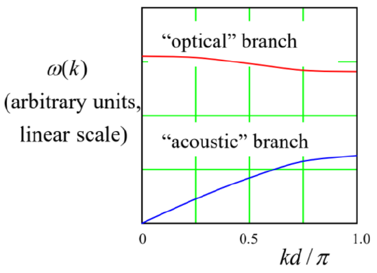
Note, however, that when a genius such as Albert Einstein makes an error, there is usually some deep and important background under it. Indeed, crystals with the basic cell consisting of atoms of two or more types (such as NaCl, etc.), feature two or more separate branches of the dispersion law \(\omega (k)\) – see, e.g., Figure \(\PageIndex{5}\). While the lower, “acoustic” branch is virtually similar to those for monoatomic crystals and may be approximated by the Debye model, \(\omega = vk\), reasonably well, the upper (“optical”⁶⁰) branch does not approach \(\omega = 0\) at any \(k\). Moreover, for large values of the atomic mass ratio \(r\), the optical branches are almost flat, with virtually \(k\)-independent frequencies \(\omega_0\), which correspond to simple oscillations of each light atom between its heavy neighbors. For thermal excitations of such oscillations, and their contribution to the specific heat, Einstein’s model (with \(\omega_E = \omega_0\)) gives a very good approximation, so that for such solids, the specific heat may be well described by a sum of the Debye and Einstein laws (\ref{97}) and (\ref{101}), with appropriate weights.

Figure \(\PageIndex{5}\): The dispersion relation for mechanical waves in a simple 1D model of a solid, with similar interparticle distances d, but alternating particle masses, plotted for a particular mass ratio \(r = 5\) – see CM Chapter 6.