
2.7: Grand canonical ensemble and distribution


- Last updated
- Sep 20, 2022
- Save as PDF

( \newcommand{\kernel}{\mathrm{null}\,}\)
As we have seen, the Gibbs distribution is a very convenient way to calculate the statistical and thermodynamic properties of systems with a fixed number N of particles. However, for systems in which N may vary, another distribution is preferable for applications. Several examples of such situations (as well as the basic thermodynamics of such systems) have already been discussed in Sec. 1.5. Perhaps even more importantly, statistical distributions for systems with variable N are also applicable to some ensembles of independent particles in certain single-particle states even if the number of the particles is fixed – see the next section.
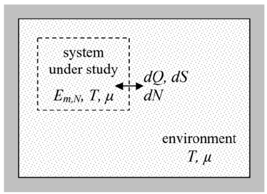
With this motivation, let us consider what is called the grand canonical ensemble (Figure \PageIndex{1}). It is similar to the canonical ensemble discussed in Sec. 4 (see Figure 2.4.1) in all aspects, besides that now the system under study and the heat bath (in this case more often called the environment) may exchange not only heat but also particles. In this ensemble, all environments are in both the thermal and chemical equilibrium, with their temperatures T and chemical potentials \mu the same for all members.
Let us assume that the system of interest is also in the chemical and thermal equilibrium with its environment. Then using exactly the same arguments as in Sec. 4 (including the specification of microcanonical sub-ensembles with fixed E_{\Sigma} and N_{\Sigma} ), we may generalize Equation (2.4.4), taking into account that the entropy S_{env} of the environment is now a function of not only its energy E_{env} = E_{\Sigma} – E_{m,N}, 61 but also of the number of particles N_{env} = N_{\Sigma} – N, with E_{\Sigma} and N_{\Sigma} fixed:
\begin{align} &\ln W_{m, N} \propto \ln M=\ln g_{env}\left(E_{\Sigma}-E_{m, N}, N_{\Sigma}-N\right)+\ln \Delta E_{\Sigma}=S_{env}\left(E_{\Sigma}-E_{m, N}, N_{\Sigma}-N\right)+\text { const } \nonumber\\ &\approx S_{env}\left|E_{\Sigma}, N_{\Sigma}-\frac{\partial S_{env}}{\partial E_{env}} \right|_{E_{\Sigma}, N_{\Sigma}} E_{m, N}- \left. \frac{\partial S_{env}}{\partial N_{env}} \right|_{E_{\Sigma}, N_{\Sigma}} N +\text{ const. } \label{102}\end{align}
To simplify this relation, let us rewrite Equation (1.5.1) in the following equivalent form:
dS = \frac{1}{T} dE + \frac{P}{T} dV - \frac{\mu}{T} dN. \label{103}
Hence, if the entropy S of a system is expressed as a function of E, V, and N, then
\left(\frac{\partial S}{\partial E}\right)_{V,N} = \frac{1}{T}, \quad \left(\frac{\partial S}{\partial V}\right)_{E,N} = \frac{P}{T}, \quad \left(\frac{\partial S}{\partial N}\right)_{E,V} = -\frac{\mu }{T}. \label{104}
Applying the first one and the last one of these relations to the last form of Equation (\ref{102}), and using the equality of the temperatures T and chemical potentials \mu in the system under study and its environment, at equilibrium (as was discussed in Sec. 1.5), we get
\ln W_{m,N} = S_{env} (E_{\Sigma},N_{\Sigma}) - \frac{1}{T} E_{m,N} + \frac{\mu}{T} N+ \text{const}. \label{105}
Again, exactly as at the derivation of the Gibbs distribution in Sec. 4, we may argue that since E_{m,N}, T, and \mu do not depend on the choice of environment’s size, i.e. on E_{\Sigma} and N_{\Sigma}, the probability W_{m,N} for a system to have N particles and be in m^{th} quantum state in the whole grand canonical ensemble should also obey Equation (\ref{105}). As a result, we get the so-called grand canonical distribution:
Grand canonical distribution:
\boxed{W_{n,N} = \frac{1}{Z_G} \text{exp}\left\{ \frac{\mu N-E_{m,N}}{T}\right\}.} \label{106}
Just as in the case of the Gibbs distribution, the constant Z_G (most often called the grand statistical sum, but sometimes the “grand partition function”) should be determined from the probability normalization condition, now with the summation of probabilities W_{m,N} over all possible values of both m and N:
Grand canonical sum:
\boxed{Z_G = \sum_{m,N} \text{exp}\left\{\frac{\mu N-E_{m,N}}{T}\right\}.} \label{107}
Now, using the general Equation (2.2.11) to calculate the entropy for the distribution (\ref{106}) (exactly like we did it for the canonical ensemble), we get the following expression,
S = - \sum_{m,N} W_{m,N} \ln W_{m,N} = \frac{E}{T} - \frac{\mu \langle N \rangle}{T} + \ln Z_G, \label{108}
which is evidently a generalization of Equation (2.4.12).62 We see that now the grand thermodynamic potential \Omega (rather than the free energy F) may be expressed directly via the normalization coefficient Z_G:
\boldsymbol{\Omega} from \mathbf{Z_G}:
\boxed{\Omega \equiv F-\mu\langle N\rangle=E-T S-\mu\langle N\rangle=T \ln \frac{1}{Z_{\mathrm{G}}}=-T \ln \sum_{m, N} \exp \left\{\frac{\mu N-E_{m, N}}{T}\right\}.} \label{109}
Finally, solving the last equality for Z_G, and plugging the result back into Equation (\ref{106}), we can rewrite the grand canonical distribution in the form
W_{m,N} = \text{exp}\left\{ \frac{\Omega + \mu N - E_{m,N}}{T}\right\}, \label{110}
similar to Equation (2.4.15) for the Gibbs distribution. Indeed, in the particular case when the number N of particles is fixed, N = \langle N\rangle , so that \Omega + \mu N = \Omega + \mu \langle N\rangle \equiv F, Equation (\ref{110}) is reduced to Equation (2.4.15).