2.9: Exercise problems

Exercise \(\PageIndex{1}\)

A famous example of macroscopic irreversibility was suggested in 1907 by P. Ehrenfest. Two dogs share \(2N >> 1\) fleas. Each flea may jump onto another dog, and the rate \(\Gamma\) of such events (i.e. the probability of jumping per unit time) does not depend either on time or on the location of other fleas. Find the time evolution of the average number of fleas on a dog, and of the flea-related part of the total dogs’ entropy (at arbitrary initial conditions), and prove that the entropy can only grow.⁶⁹

Exercise \(\PageIndex{2}\)

Use the microcanonical distribution to calculate thermodynamic properties (including the entropy, all relevant thermodynamic potentials, and the heat capacity), of a two-level system in thermodynamic equilibrium with its environment, at temperature \(T\) that is comparable with the energy gap \(\Delta \). For each variable, sketch its temperature dependence, and find its asymptotic values (or trends) in the low-temperature and high-temperature limits.

Exercise \(\PageIndex{3}\)

Solve the previous problem using the Gibbs distribution. Also, calculate the probabilities of the energy level occupation, and give physical interpretations of your results, in both temperature limits.

Exercise \(\PageIndex{4}\)

Calculate low-field magnetic susceptibility \(\chi\) of a quantum spin-1/2 particle with a gyromagnetic ratio \(\gamma \), in thermal equilibrium with an environment at temperature \(T\), neglecting its orbital motion. Compare the result with that for a classical spontaneous magnetic dipole \(\pmb{\mathscr{m}}\) of a fixed magnitude \(\mathscr{m}_0\), free to change its direction in space.

Hint: The low-field magnetic susceptibility of a single particle is defined⁷¹ as

\[\xi = \frac{\partial \langle \mathscr{m}_z \rangle}{\partial \mathscr{H}} \mid_{\mathscr{H}\to0},\nonumber\]

where the \(z\)-axis is aligned with the direction of the external magnetic field \(\pmb{\mathscr{H}}\).

Exercise \(\PageIndex{5}\)

Calculate the low-field magnetic susceptibility of a particle with an arbitrary (either integer or semi-integer) spin \(s\), neglecting its orbital motion. Compare the result with the solution of the previous problem.

Hint: Quantum mechanics⁷² tells us that the Cartesian component \(\mathscr{m}_z\) of the magnetic moment of such a particle, in the direction of the applied field, has \((2s + 1)\) stationary values:

\[\mathscr{m}_z=\gamma\hbar m_s, \quad \text{ with } m_s = -s, -s+1,...,s-1,s, \nonumber\]

where \(\gamma\) is the gyromagnetic ratio of the particle, and \(\hbar\) is Planck’s constant.

Exercise \(\PageIndex{6}\)*

Analyze the possibility of using a system of non-interacting spin-1/2 particles, placed into a strong, controllable external magnetic field, for refrigeration.

Exercise \(\PageIndex{7}\)

The rudimentary “zipper” model of DNA replication is a chain of \(N\) links that may be either open or closed – see the figure on the right.

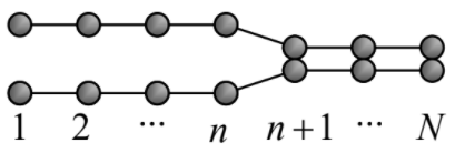
Opening a link increases the system’s energy by \(\Delta > 0\); a link may change its state (either open or closed) only if all links to the left of it are open, while those on the right of it, are closed. Calculate the average number of open links at thermal equilibrium, and analyze its temperature dependence, especially for the case \(N >> 1\).

Exercise \(\PageIndex{8}\)

Use the microcanonical distribution to calculate the average entropy, energy, and pressure of a classical particle of mass \(m\), with no internal degrees of freedom, free to move in volume \(V\), at temperature \(T\).

Hint: Try to make a more accurate calculation than has been done in Sec. 2.2 for the system of \(N\) harmonic oscillators. For that, you will need to know the volume \(V_d\) of a \(d\)-dimensional hypersphere of the unit radius. To avoid being too cruel, I am giving it to you:

\[V_d = \pi^{d/2} / \Gamma \left(\frac{d}{2}+1\right), \nonumber\]

where \(\Gamma (\xi )\) is the gamma function.⁷³

Exercise \(\PageIndex{9}\)

Solve the previous problem starting from the Gibbs distribution.

Exercise \(\PageIndex{10}\)

Calculate the average energy, entropy, free energy, and the equation of state of a classical 2D particle (without internal degrees of freedom), free to move within area \(A\), at temperature \(T\), starting from:

(i) the microcanonical distribution, and

(ii) the Gibbs distribution.

Hint: For the equation of state, make the appropriate modification of the notion of pressure.

Exercise \(\PageIndex{11}\)

A quantum particle of mass \(m\) is confined to free motion along a 1D segment of length \(a\). Using any approach you like, calculate the average force the particle exerts on the “walls” (ends) of such “1D potential well” in thermal equilibrium, and analyze its temperature dependence, focusing on the low-temperature and high-temperature limits.

Hint: You may consider the series \(\Theta(\xi) \equiv \sum_{n=1}^{\infty} \exp \left\{-\xi n^{2}\right\}\) a known function of \(\xi \). ⁷⁴

Exercise \(\PageIndex{12}\)*

Rotational properties of diatomic molecules (such as \(\ce{N2}\), CO, etc.) may be reasonably well described by the so-called dumbbell model: two point particles, of masses \(m_1\) and \(m_2\), with a fixed distance \(d\) between them. Ignoring the translational motion of the molecule as the whole, use this model to calculate its heat capacity, and spell out the result in the limits of low and high temperatures. Discuss whether your solution is valid for the so-called homonuclear molecules, consisting of two similar atoms, such as \(\ce{H2}\), \(\ce{O2}\), \(\ce{N2}\), etc.

Exercise \(\PageIndex{13}\)

Calculate the heat capacity of a heteronuclear diatomic molecule, using the simple model described in the previous problem, but now assuming that the rotation is confined to one plane.⁷⁵

Exercise \(\PageIndex{14}\)

A classical, rigid, strongly elongated body (such as a thin needle), is free to rotate about its center of mass, and is in thermal equilibrium with its environment. Are the angular velocity vector \(\omega\) and the angular momentum vector \(\mathbf{L}\), on average, directed along the elongation axis of the body, or normal to it?

Exercise \(\PageIndex{15}\)

Two similar classical electric dipoles, of a fixed magnitude \(d\), are separated by a fixed distance \(r\). Assuming that each dipole moment \(\mathbf{d}\) may take any spatial direction and that the system is in thermal equilibrium, write the general expressions for its statistical sum \(Z\), average interaction energy \(E\), heat capacity \(C\), and entropy \(S\), and calculate them explicitly in the high-temperature limit.

Exercise \(\PageIndex{16}\)

A classical 1D particle of mass \(m\), residing in the potential well

\[U(x) = \alpha |x|^{\gamma}, \quad \text{ with } \gamma >0, \nonumber\]

is in thermal equilibrium with its environment, at temperature \(T\). Calculate the average values of its potential energy \(U\) and the full energy \(E\), using two approaches:

(i) directly from the Gibbs distribution, and

Exercise \(\PageIndex{17}\)

For a thermally-equilibrium ensemble of slightly anharmonic classical 1D oscillators, with mass \(m\) and potential energy

\[U(q) = \frac{\kappa}{2}x^2 + \alpha x^3, \nonumber\]

with a small coefficient \(\alpha \), calculate \(\langle x\rangle\) in the first approximation in low temperature \(T\).

Exercise \(\PageIndex{18}\)*

A small conductor (in this context, usually called the single-electron island) is placed between two conducting electrodes, with voltage \(V\) applied between them. The gap between one of the electrodes and the island is so narrow that electrons may tunnel quantum-mechanically through this gap (the “weak tunnel junction”) – see the figure on the right. Calculate the average charge of the island as a function of \(V\) at temperature \(T\).

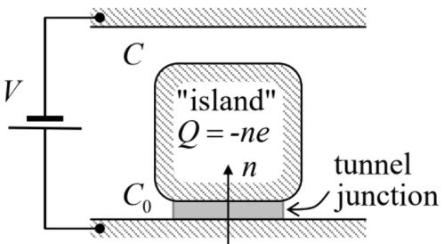
Hint: The quantum-mechanical tunneling of an electron through a weak junction⁷⁷ between two macroscopic conductors and their subsequent energy relaxation, may be considered as a single inelastic (energy-dissipating) event, so that the only energy relevant for the thermal equilibrium of the system is its electrostatic potential energy.

Exercise \(\PageIndex{19}\)

An \(LC\) circuit (see the figure on the right) is in thermodynamic equilibrium with its environment. Calculate the r.m.s. fluctuation \(\delta V \equiv \langle V^2 \rangle^{1/2}\) of the voltage across it, for an arbitrary ratio \(T/\hbar \omega \), where \(\omega = (LC)^{-1/2}\) is the resonance frequency of this “tank circuit”.

Exercise \(\PageIndex{20}\)

Derive Equation (\(2.6.12-2.6.13\)) from simplistic arguments, representing the blackbody radiation as an ideal gas of photons treated as classical ultra-relativistic particles. What do similar arguments give for an ideal gas of classical but non-relativistic particles?

Exercise \(\PageIndex{21}\)

Calculate the enthalpy, the entropy, and the Gibbs energy of blackbody electromagnetic radiation with temperature \(T\) inside volume \(V\), and then use these results to find the law of temperature and pressure drop at an adiabatic expansion.

Exercise \(\PageIndex{22}\)

As was mentioned in Sec. 6(i), the relation between the temperatures \(T_{\oplus}\) of the visible Sun’s surface and that \((T_o)\) of the Earth’s surface follows from the balance of the thermal radiation they emit. Prove that the experimentally observed relation indeed follows, with good precision, from a simple model in which the surfaces radiate as perfect black bodies with constant temperatures.

Hint: You may pick up the experimental values you need from any (reliable :-) source.

Exercise \(\PageIndex{23}\)

If a surface is not perfectly radiation-absorbing (“black”), the electromagnetic power of its thermal radiation differs from the Planck radiation law by a frequency-dependent factor \(\varepsilon < 1\), called the emissivity. Prove that such surface reflects the (\(1 – \varepsilon \)) fraction of the incident radiation.

Exercise \(\PageIndex{24}\)

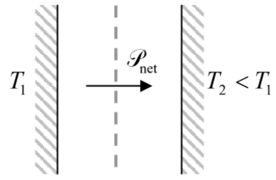
If two black surfaces, facing each other, have different temperatures (see the figure on the right), then according to the Stefan radiation law (\(2.6.8-2.6.9\)), there is a net flow of thermal radiation, from a warmer surface to the colder one:

\[\frac{\mathscr{P}_{net}}{A} = \sigma (T^4_1 - T^4_2). \nonumber\]

For many applications, notably including most low-temperature experiments, this flow is detrimental. One way to suppress it is to reduce the emissivity \(\varepsilon\) (for its definition, see the previous problem) of both surfaces – say by covering them with shiny metallic films. An alternative way toward the same goal is to place, between the surfaces, a thin layer (usually called the thermal shield), with a low emissivity of both surfaces – see the dashed line in Figure above. Assuming that the emissivity is the same in both cases, find out which way is more efficient.

Exercise \(\PageIndex{25}\)

Two parallel, well-conducting plates of area \(A\) are separated by a free-space gap of a constant thickness \(t << A^{1/2}\). Calculate the energy of the thermally-induced electromagnetic field inside the gap at thermal equilibrium with temperature \(T\) in the range

\[\frac{\hbar c}{A^{1/2}} <<T<<\frac{\hbar c}{t}. \nonumber\]

Does the field push the plates apart?

Exercise \(\PageIndex{26}\)

Use the Debye theory to estimate the specific heat of aluminum at room temperature (say, 300 K), and express the result in the following popular units:

(i) eV/K per atom,

(ii) J/K per mole, and

(iii) J/K per gram.

Compare the last number with the experimental value (from a reliable book or online source).

Exercise \(\PageIndex{27}\)

Low-temperature specific heat of some solids has a considerable contribution from thermal excitation of spin waves, whose dispersion law scales as \(\omega \propto k^2\) at \(\omega \rightarrow 0\).⁷⁸ Neglecting anisotropy, calculate the temperature dependence of this contribution to \(C_V\) at low temperatures, and discuss conditions of its experimental observation.

Hint: Just as the photons and phonons discussed in section 2.6, the quantum excitations of spin waves (called magnons) may be considered as non-interacting bosonic quasiparticles with zero chemical potential, whose statistics obeys Equation (\(2.5.15\)).

Exercise \(\PageIndex{28}\)

Derive a general expression for the specific heat of a very long, straight chain of similar particles of mass \(m\), confined to move only in the direction of the chain, and elastically interacting with effective spring constants \(\kappa\) – see the figure on the right. Spell out the result in the limits of very low and very high temperatures.

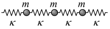
Hint: You may like to use the following integral:⁷⁹

\[\int^{+\infty}_{0} \frac{\xi^2 d \xi}{\sinh^2 \xi} = \frac{\pi^2}{6}.\nonumber\]

Exercise \(\PageIndex{29}\)

Calculate the r.m.s. thermal fluctuation of the middle point of a uniform guitar string of length \(l\), stretched by force \(\mathscr{T}\), at temperature \(T\). Evaluate your result for \(l = 0.7\) m, \(\mathscr{T} = 10^3\) N, and room temperature.

Hint: You may like to use the following series:

\[1+\frac{1}{3^2}+\frac{1}{5^2}+...\equiv \sum^{\infty}_{m\to 0} \frac{1}{(2m+1)^2} = \frac{\pi^2}{8}.\nonumber\]

Exercise \(\PageIndex{30}\)

Use the general Equation (\(2.8.13\)) to re-derive the Fermi-Dirac distribution (\(2.8.5\)) for a system in equilibrium.

Exercise \(\PageIndex{31}\)

Each of two identical particles, not interacting directly, may be in any of two quantum states, with single-particle energies \(\varepsilon\) equal to 0 and \(\Delta \). Write down the statistical sum \(Z\) of the system, and use it to calculate its average total energy \(E\) at temperature \(T\), for the cases when the particles are:

(i) distinguishable (say, by their positions);

(ii) indistinguishable fermions;

(iii) indistinguishable bosons.

Analyze and interpret the temperature dependence of \(E\) for each case, assuming that \(\Delta > 0\).

Exercise \(\PageIndex{32}\)

Calculate the chemical potential of a system of \(N >> 1\) independent fermions, kept at a fixed temperature \(T\), if each particle has two non-degenerate energy levels separated by gap \(\Delta \).

---

Footnotes

1. For the reader interested in a more rigorous approach, I can recommend, for example, Chapter 18 of the handbook by G. Korn and T. Korn – see MA Sec. 16(ii).
2. The most popular counter-example is an energy-conserving system. Consider, for example, a system of particles placed in a potential that is a quadratic form of its coordinates. The theory of oscillations tells us (see, e.g., CM Sec. 6.2) that this system is equivalent to a set of non-interacting harmonic oscillators. Each of these oscillators conserves its own initial energy \(E_j\) forever, so that the statistics of \(N\) measurements of one such system may differ from that of \(N\) different systems with a random distribution of \(E_j\), even if the total energy of the system, \(E = \Sigma_jE_j\), is the same. Such non-ergodicity, however, is a rather feeble phenomenon and is readily destroyed by any of many mechanisms, such as weak interaction with the environment (leading, in particular, to oscillation damping), potential anharmonicity (see, e.g., CM Chapter 5), and chaos (CM Chapter 9), all of them strongly enhanced by increasing the number of particles in the system, i.e. the number of its degrees of freedom. This is why an overwhelming part of real-life systems are ergodic; for the readers interested in non-ergodic exotics, I can recommend the monograph by V. Arnold and A. Avez, Ergodic Problems of Classical Mechanics, Addison Wesley, 1989.
3. Here, and everywhere in this series, angle brackets \(\langle \dots \rangle\) mean averaging over a statistical ensemble, which is generally different from averaging over time – as it will be the case in quite a few examples considered below.
4. See, e.g., QM Sec. 7.1.
5. Here I use the Schrödinger picture of quantum dynamics, in which the matrix elements \(f_{nn’}\) representing quantum-mechanical operators, do not evolve in time. The final results of this discussion do not depend on the particular picture – see, e.g., QM Sec. 4.6.
6. Personally, I believe that the genius of J. Gibbs, praised by Albert Einstein as the “greatest mind in the American history”, is still insufficiently recognized, and agree with R. Millikan that Gibbs “did for statistical mechanics and thermodynamics what [...] Maxwell did for electrodynamics”.
7. The terms “microcanonical”, as well as “canonical” (see Sec. 4 below) are apparently due to Gibbs and I was unable to find out his motivation for the former name. (“Canonical” in the sense of “standard” or “common” is quite appropriate, but why “micro”? Perhaps to reflect the smallness of \(\Delta E\)?)
8. Formally, the main result of this section, Equation (\(2.2.1\)), is valid for any \(M\) (including \(M = 1\)); it is just less informative for small \(M\) – and trivial for \(M = 1\).
9. Though I have to move on, let me note that the microcanonical distribution (\(2.2.1\)) is a very nontrivial postulate, and my advice to the reader is to find some time to give additional thought to this keystone of the whole building of statistical mechanics.
10. I will rely on the reader’s common sense and intuitive understanding of what information is, because even in the formal information theory, this notion is essentially postulated – see, e.g., the wonderfully clear text by J. Pierce, An Introduction to Information Theory, Dover, 1980.
11. This is of course just the change of a constant factor: \(S(M) = \ln M = \ln 2 \times \log_2M = \ln 2 \times I(M) \approx 0.693 I(M)\). A review of Chapter 1 shows that nothing in thermodynamics prevents us from choosing such a constant coefficient arbitrarily, with the corresponding change of the temperature scale – see Equation (1.9). In particular, in the SI units, where Equation (\(2.2.6\)) becomes \(S = –k_B \ln W_m\), one bit of information corresponds to the entropy change \(\Delta S = k_B \ln 2 \approx 0.693 k_B \approx 0.965\times 10^{-23}\) J/K. By the way, the formula “\(S = k \log W\)” is engraved on L. Boltzmann’s tombstone in Vienna.
12. See, e.g., MA Equation (2.3). Despite the intimidating name, Equation (\(2.2.8\)) may be very simply derived. Indeed, \(N\)! is just the number of all possible permutations of \(N\) balls, i.e. the ways to place them in certain positions – say, inside \(M\) boxes. Now to take into account that the particular order of the balls in each box is not important, that number should be divided by all numbers \(N_m\)! of possible permutations of balls within each box – that’s it.
13. See, e.g., MA Equation (2.10).
14. Strictly speaking, I should use the notation \(\langle S \rangle\) here. However, following the style accepted in thermodynamics, I will drop the averaging signs until we will really need them to avoid confusion. Again, this shorthand is not too bad because the relative fluctuations of entropy (as those of any macroscopic variable) are very small at \(N >> 1\).
15. With the replacement of \(\ln W_m\) with \(\log_2 W_m\) (i.e. division of both sides by \(\ln 2\)), Equation (\(2.2.11\)) becomes the famous Shannon (or “Boltzmann-Shannon”) formula for the average information \(I\) per symbol in a long communication string using \(M\) different symbols, with probability \(W_m\) each.
16. In some textbooks, this interpretation is even accepted as the derivation of Equation (\(2.2.11\)); however, it is evidently less strict than the one outlined above.
17. See, e.g., QM Secs. 2.9 and 5.4.
18. Let me hope that the reader knows that the ground-state energy is experimentally measurable – for example, using the famous Casimir effect – see, e.g., QM Sec. 9.1. (In Sec. 5.5 below I will briefly discuss another method of experimental observation of that energy.)
19. The coefficient \(1/N\)! in this formula has the geometrical meaning of the (hyper)volume of the \(N\)-dimensional right pyramid with unit sides.
20. For the same reason, the notion of pressure \(P\) in such a system is not clearly defined, and neither are any thermodynamic potentials but \(E\) and \(F\).
21. I am using this fancy font for the mass to avoid any chance of its confusion with the state number.
22. Note again that while we have committed the energy \(E_N\) of \(N\) oscillators to be fixed (to apply Equation (\(2.2.18\)), valid only for a microcanonical ensemble at thermodynamic equilibrium), the single oscillator’s energy \(E\) in our analysis may be arbitrary – within the limits \(\hbar \omega << E \leq E_N \sim NT\).
23. As a reminder, the Hamiltonian of any system whose classical Lagrangian function is an arbitrary quadratic form of its generalized coordinates and the corresponding generalized velocities, may be brought to the form (\(2.2.31\)) by an appropriate choice of “normal coordinates” \(q_j\) which are certain linear combinations of the original coordinates – see, e.g., CM Sec. 6.2.
24. This also means that in the classical limit, the heat capacity of a system is equal to one-half of the number of its half-degrees of freedom (in the SI units, multiplied by \(k_B\)).
25. The reader is strongly urged to solve Problem 2, whose task is to do a similar calculation for another key (“two level”) physical system, and compare the results.
26. See, e.g., CM Chapter 9 and literature therein.
27. For the definition of \(\lambda \), see, e.g., CM Equation (9.9).
28. For more discussion, see, e.g., either Sec. 6.2 of the monograph H. G. Schuster and W. Just, Deterministic Chaos, \(4^{th}\) ed., Wiley-VHS, 2005, or the monograph by Arnold and Avez, cited in Sec. 1.
29. This system is frequently called the Szilard engine, after L. Szilard who published its detailed theoretical discussion in 1929, but is essentially a straightforward extension of the thought experiment suggested by J. Maxwell as early as 1867.
30. This procedure of the statistical ensemble re-definition is the central point of the connection between physics and information theory, and is crucial in particular for any (or rather any meaningful :-) discussion of measurements in quantum mechanics – see, e.g., QM Secs. 2.5 and 10.1.
31. See, for example, A. Bérut et al., Nature 483, 187 (2012); J. Koski et al., PNAS USA 111, 13786 (2014); Y. Jun et al., Phys. Rev. Lett. 113, 190601 (2014); J. Peterson et al., Proc. Roy. Soc. A 472, 20150813 (2016).
32. C. Bennett, IBM J. Res. Devel. 17, 525 (1973); see also C. Bennett, Int. J. Theor. Phys. 21, 905 (1982).
33. For that, all gates have to be physically reversible, with no static power consumption. Such logic devices do exist, though they are still not very practicable – see, e.g., K. Likharev, Int. J. Theor. Phys. 21, 311 (1982). (Another reason for citing, rather reluctantly, my own paper is that it also gave constructive proof that the reversible computation may also beat the perceived “fundamental quantum limit”, \(\Delta E\Delta t > \hbar \), where \(\Delta t\) is the time of the binary logic operation.)
34. Many currently explored schemes of quantum computing are also reversible – see, e.g., QM Sec. 8.5 and references therein.
35. Another famous example is Charles Darwin’s theory of biological evolution.
36. The temperature dependence of the type \(\text{exp}\{-const/T\}\), especially when showing up in rates of certain events, e.g., chemical reactions, is also frequently called the Arrhenius law – after chemist S. Arrhenius who has noticed this law in numerous experimental data. In all cases I am aware of, the Gibbs distribution is the underlying reason of the Arrhenius law. (We will see several examples of that later in this course.)
37. This is the opinion of many physicists, including Richard Feynman – who climbs on this “summit” already on the first page of his brilliant book Statistical Mechanics, CRC Press, 1998. (This is a collection of lectures on a few diverse, mostly advanced topics of statistical physics, rather than its systematic course, so that it can hardly be used as the first textbook on the subject. However, I can highly recommend its first chapter to all my readers.
38. The task of making a similar (and even simpler) calculation for another key quantum-mechanical object, the two-level system, is left for the reader’s exercise.
39. See, e.g., MA Equation (2.8b).
40. It was first obtained in 1924 by S. Bose and is sometimes called the Bose distribution – a particular case of the Bose-Einstein distribution to be discussed in Sec. 8 below.
41. See, e.g., QM Sec. 2.10.
42. The calculation may be found, e.g., in QM Sec. 7.2.
43. As a reminder: the equality of these two averages, at arbitrary temperature, was proved already in Sec. 2.
44. See, e.g., EM Sec. 7.8.
45. In our current context, the volume should be much larger than \((c\hbar /T)^3\), where \(c \approx 3\times 10^8\) m/s is the speed of light. For the room temperature (\(T \approx k_B \times 300\) K \(\approx 4\times 10^{-21}\) J), this lower bound is of the order of \(10^{-16} m^3\).
46. See, e.g., QM Sec. 9.1.
47. Let me hope the reader knows that this law was first suggested in 1900 by Max Planck as an empirical fit for the experimental data on blackbody radiation, and this was the historic point at which the Planck constant \(\hbar\) (or rather \(h \equiv 2\pi \hbar \)) was introduced – see, e.g., QM Sec. 1.1.
48. The last step in Equation (\(2.6.7\)) uses a table integral, equal to \(\Gamma (4)\zeta (4) = (3!)(\pi^4/90) = \pi^4/15\) – see, e.g., MA Equation (6.8b), with \(s = 4\), and then MA Eqs. (6.7e), and (2.7b).
49. Note that the heat capacity \(C_V \equiv (\partial E/\partial T)_V\), following from Equation (\(2.6.7\)), is proportional to \(T^3\) at any temperature, and hence does not obey the trend \(C_V \rightarrow\) const at \(T \rightarrow \infty \). This is the result of the unlimited growth, with temperature, of the number of thermally-exited field oscillators with frequencies \(\omega\) below \(T/\hbar \).
50. Its functional part \((E \propto T^4)\) was deduced in 1879 by Joseph Stefan from earlier experiments by John Tyndall. Theoretically, it was proved in 1884 by L. Boltzmann, using a result derived earlier by Adolfo Bartoli from the Maxwell equations for the electromagnetic field – all well before Max Planck’s work.
51. This formula may be also derived from the expression for the forces exerted by the electromagnetic radiation on the walls (see, e.g. EM Sec. 9.8), but the above calculation is much simpler.
52. Note that according to Eqs. (\(1.4.21\)), (\(2.6.7\)), and (\(2.6.12-2.6.13\)), the difference between the equations of state of the photon gas and an ideal gas of non-relativistic particles, expressed in the more usual form \(P = P(V, T)\), is much more dramatic: \(P \propto T^4V^0\) vs. \(P \propto T^1V^{-1}\).
53. Due to a rather low temperature expansion of solids, the difference between their \(C_V\) and \(C_P\) is small.
54. In good conductors (e.g., metals), specific heat is contributed (and at low temperatures, dominated) by free electrons – see Sec. 3.3 below.
55. See, e.g., CM Sec. 7.7.
56. See, e.g., CM Sec. 6.3, in particular Figure 6.5 and its discussion.
57. See, e.g., CM Sec. 6.2.
58. In the SI units, the Debye temperature \(T_D\) is of the order of a few hundred K for most simple solids (e.g., \(\sim 430\) K for aluminum and \(\sim 340\) K for copper), with somewhat lower values for crystals with heavy atoms (\(\sim 105\) K for lead), and reaches its highest value \(\sim 2200\) K for diamond, with its relatively light atoms and very stiff lattice.
59. This is why there is the following general “rule of thumb” in quantitative sciences: if you plot your data on a linear rather than log scale, you better have a good excuse ready. (An example of a valid excuse: the variable you are plotting changes its sign within the range you want to exhibit.)
60. This term stems from the fact that at \(k \rightarrow 0\), the mechanical waves corresponding to these branches have phase velocities \(v_{ph} \equiv \omega (k)/k\) that are much higher than that of the acoustic waves, and may approach the speed of light. As a result, these waves can strongly interact with electromagnetic (practically, optical) waves of the same frequency, while acoustic waves cannot.
61. The additional index in the new notation \(E_{m,N}\) for the energy of the system of interest reflects the fact that its spectrum is generally dependent on the number \(N\) of particles in it.
62. The average number of particles \(\langle N\rangle\) is exactly what was called \(N\) in thermodynamics (see Chapter 1), but I keep this explicit notation here to make a clear distinction between this average value of the variable, and its particular values participating in Eqs. (\(2.7.1\))-(\(2.7.10\)).
63. The distribution was first suggested in 1877 by L. Boltzmann. For the particular case when \(\varepsilon\) is the kinetic energy of a free classical particle (and hence has a continuous spectrum), it is reduced to the Maxwell distribution (see Sec. 3.1 below), which was derived earlier – in 1860.
64. This invites a natural question: what particles are “elementary enough” for their identity? For example, protons and neutrons have an internal structure, in some sense consisting of quarks and gluons; can they be considered elementary? Next, if protons and neutrons are elementary, are atoms? molecules? What about really large molecules (such as proteins)? viruses? The general answer to these questions, given by quantum mechanics (or rather experiment :-), is that any particles/systems, no matter how large and complex they are, are identical if they not only have the same internal structure but also are exactly in the same internal quantum state – for example, in the ground state of all their internal degrees of freedom.
65. For a more detailed discussion of this issue, see, e.g., QM Sec. 8.1.
66. As the reader certainly knows, for the electromagnetic field oscillators, such excitations are called photons; for mechanical oscillation modes, phonons. It is important, however, not to confuse these mode excitations with the oscillators as such, and be very careful in prescribing to them certain spatial locations – see, e.g., QM Sec. 9.1.
67. See, e.g., MA Equation (2.2).
68. See also MA Equation (2.4).
69. This is essentially a simpler (and funnier :-) version of the particle scattering model used by L. Boltzmann to prove his famous \(H\)-theorem (1872). Besides the historic significance of that theorem, the model used in it (see Sec. 6.2 below) is as cartoonish, and not more general.
70. See, e.g., QM Secs. 4.6 and 5.1, for example, Equation (4.167).
71. This “atomic” (or “molecular”) susceptibility should be distinguished from the “volumic” susceptibility \(\chi_m \equiv \partial \mathscr{M}_z/\partial \mathscr{H}\), where \(\pmb{\mathscr{M}}\) is the magnetization, i.e. the magnetic moment of a unit volume of a system – see, e.g., EM Equation (5.111). For a uniform medium with \(n \equiv N/V\) non-interacting dipoles per unit volume, \(\chi_m = n\chi \).
72. See, e.g., QM Sec. 5.7, in particular Equation (5.169).
73. For its definition and main properties, see, e.g., MA Eqs. (6.6)-(6.9).
74. It may be reduced to the so-called elliptic theta-function \(\theta_3 (z, \tau )\) for a particular case \(z = 0\) – see, e.g., Sec. 16.27 in the Abramowitz-Stegun handbook cited in MA Sec. 16(ii). However, you do not need that (or any other) handbook to solve this problem.
75. This is a reasonable model of the constraints imposed on small atomic groups (e.g., ligands) by their atomic environment inside some large molecules.
76. See, e.g., CM Problem 1.12.
77. In this particular context, the adjective “weak” denotes a junction with the tunneling transparency so low that the tunneling electron’s wavefunction loses its quantum-mechanical coherence before the electron has a chance to tunnel back. In a typical junction of a macroscopic area this condition is fulfilled if its effective resistance is much higher than the quantum unit of resistance (see, e.g., QM Sec. 3.2), \(R_Q \equiv \pi \hbar /2e^2 \approx 6.5\) k\(\Omega \).
78. Note that the same dispersion law is typical for bending waves in thin elastic rods – see, e.g., CM Sec. 7.8.
79. It may be reduced, via integration by parts, to the table integral MA Equation (6.8d) with \(n = 1\).