
3.6: Exercise problems


- Last updated
- Sep 20, 2022
- Save as PDF

( \newcommand{\kernel}{\mathrm{null}\,}\)
Use the Maxwell distribution for an alternative (statistical) calculation of the mechanical work performed by the Szilard engine discussed in Sec. 2.3.
Hint: You may assume the simplest geometry of the engine – see Figure 2.3.1.
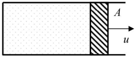
Use the Maxwell distribution to calculate the drag coefficient η≡–∂⟨F⟩/∂u, where F is the force exerted by an ideal classical gas on a piston moving with a low velocity u, in the simplest geometry shown in the figure on the right, assuming that collisions of gas particles with the piston are elastic.
Derive the equation of state of the ideal classical gas from the grand canonical distribution.
Prove that Equation (3.1.23),
ΔS=N1lnV1+V2V1+N2lnV1+V2V2,
derived for the change of entropy at mixing of two ideal classical gases of completely distinguishable particles (that initially had equal densities N/V and temperatures T), is also valid if particles in each of the initial volumes are indistinguishable from each other but different from those in the counterpart volume. For simplicity, you may assume that masses and internal degeneracy factors of all particles are equal.
A round cylinder of radius R and length L, containing an ideal classical gas of N>>1 particles of mass m each, is rotated about its symmetry axis with angular velocity ω. Assuming that the gas as the whole rotates with the cylinder, and is in thermal equilibrium at temperature T,
(i) calculate the gas pressure distribution along its radius, and analyze its temperature dependence, and
(ii) neglecting the internal degrees of freedom of the particles, calculate the total energy of the gas and its heat capacity in the high- and low-temperature limits.
N>>1 classical, non-interacting, indistinguishable particles of mass m are confined in a parabolic, spherically-symmetric 3D potential well U(r)=κr2/2. Use two different approaches to calculate all major thermodynamic characteristics of the system, in thermal equilibrium at temperature T, including its heat capacity. Which of the results should be changed if the particles are distinguishable, and how?
Hint: Suggest a replacement of the notions of volume and pressure, appropriate for this system.
In the simplest model of thermodynamic equilibrium between the liquid and gas phases of the same molecules, temperature and pressure do not affect the molecule's condensation energy Δ. Calculate the concentration and pressure of such saturated vapor, assuming that it behaves as an ideal gas of classical particles.
An ideal classical gas of N>>1 particles is confined in a container of volume V and wall surface area A. The particles may condense on container walls, releasing energy Δ per particle, and forming an ideal 2D gas. Calculate the equilibrium number of condensed particles and the gas pressure, and discuss their temperature dependences.
The inner surfaces of the walls of a closed container of volume V, filled with N>>1 particles, have NS>>1 similar traps (small potential wells). Each trap can hold only one particle, at potential energy –Δ<0. Assuming that the gas of the particles in the volume is ideal and classical, derive an equation for the chemical potential μ of the system in equilibrium, and use it to calculate the potential and the gas pressure in the limits of small and large values of the N/NS ratio.
Calculate the magnetic response (the Pauli paramagnetism) of a degenerate ideal gas of spin-1/2 particles to a weak external magnetic field, due to a partial spin alignment with the field.
Calculate the magnetic response (the Landau diamagnetism) of a degenerate ideal gas of electrically charged fermions to a weak external magnetic field, due to their orbital motion.
Explore the Thomas-Fermi model of a heavy atom, with nuclear charge Q=Ze>>e, in which the electrons are treated as a degenerate Fermi gas, interacting with each other only via their contribution to the common electrostatic potential ϕ(r). In particular, derive the ordinary differential equation obeyed by the radial distribution of the potential, and use it to estimate the effective radius of the atom.50
Use the Thomas-Fermi model, explored in the previous problem, to calculate the total binding energy of a heavy atom. Compare the result with that for a simpler model, in that the Coulomb electron-electron interaction of electrons is completely ignored.
Calculate the characteristic Thomas-Fermi length λTF of weak electric field’s screening by conduction electrons in a metal, modeling their ensemble as an ideal, degenerate, isotropic Fermi gas.
Hint: Assume that λTF is much larger than the Bohr radius rB.
For a degenerate ideal 3D Fermi gas of N particles, confined in a rigid-wall box of volume V, calculate the temperature dependencies of its pressure P and the heat capacity difference (CP–CV), in the leading approximation in T<<εF. Compare the results with those for the ideal classical gas.
Hint: You may like to use the solution of Problem 1.9.
How would the Fermi statistics of an ideal gas affect the barometric formula (3.1.29)?
Derive general expressions for the energy E and the chemical potential μ of a uniform Fermi gas of N>>1 non-interacting, indistinguishable, ultra-relativistic particles.51 Calculate E, and also the gas pressure P explicitly in the degenerate gas limit T→0. In particular, is Equation (3.2.19) valid in this case?
Use Equation (3.2.20) to calculate the pressure of an ideal gas of ultra-relativistic, indistinguishable quantum particles, for an arbitrary temperature, as a function of the total energy E of the gas, and its volume V. Compare the result with the corresponding relations for the electromagnetic blackbody radiation and for an ideal gas of non-relativistic particles.
Calculate the speed of sound in an ideal gas of ultra-relativistic fermions of density n at negligible temperature.
Calculate basic thermodynamic characteristics, including all relevant thermodynamic potentials, specific heat, and the surface tension of a uniform, non-relativistic 2D electron gas with given areal density n≡N/A:
(i) at T=0, and
Calculate the effective latent heat Λef≡–N(∂Q/∂N0)N,V of evaporation of the spatially uniform Bose-Einstein condensate as a function of temperature T. Here Q is the heat absorbed by the (condensate + gas) system of N>>1 particles as a whole, while N0 is the number of particles in the condensate alone.
For an ideal, spatially-uniform Bose gas, calculate the law of the chemical potential’s disappearance at T→Tc, and use the result to prove that the heat capacity CV is a continuous function of temperature at the critical point T=Tc.
In Chapter 1 of these notes, several thermodynamic relations involving entropy have been discussed, including the first of Eqs. (1.4.16):
S=−(∂G/∂T)p.
If we combine this expression with Equation (1.5.7), G=μN, it looks like that for the Bose-Einstein condensate, whose chemical potential μ equals zero at temperatures below the critical point Tc, the entropy should vanish as well. On the other hand, dividing both parts of Equation (1.3.6) by dT, and assuming that at this temperature change the volume is kept constant, we get
CV=T(∂S/∂T)V.
(This equality was also mentioned in Chapter 1.) If the CV is known as a function of temperature, the last relation may be integrated over T to calculate S:
S=∫V=constCV(T)TdT+const.
According to Equation (3.4.11), the specific heat for the Bose-Einstein condensate is proportional to T3/2, so that the integration gives a non-zero entropy S∝T3/2. Resolve this apparent contradiction, and calculate the genuine entropy at T=Tc.
The standard analysis of the Bose-Einstein condensation, outlined in Sec. 4, may seem to ignore the energy quantization of the particles confined in volume V. Use the particular case of a cubic confining volume V=a×a×a with rigid walls to analyze whether the main conclusions of the standard theory, in particular Equation (3.4.1) for the critical temperature of the system of N>>1 particles, are affected by such quantization.
N>>1 non-interacting bosons are confined in a soft, spherically-symmetric potential well U(r)=mω2r2/2. Develop the theory of the Bose-Einstein condensation in this system; in particular, prove Equation (3.4.5), and calculate the critical temperature T∗c. Looking at the solution, what is the most straightforward way to detect the condensation in experiment?
Calculate the chemical potential of an ideal, uniform 2D gas of spin-0 Bose particles as a function of its areal density n (the number of particles per unit area), and find out whether such gas can condense at low temperatures. Review your result for the case of a large (N>>1) but finite number of particles.
Can the Bose-Einstein condensation be achieved in a 2D system of N>>1 non-interacting bosons placed into a soft, axially-symmetric potential well, whose potential may be approximated as U(r)=mω2ρ2/2, where ρ2≡x2+y2, and {x,y} are the Cartesian coordinates in the particle confinement plane? If yes, calculate the critical temperature of the condensation.
Use Eqs. (3.5.29) and (3.5.34) to calculate the third virial coefficient C(T) for the hardball model of particle interactions.
Assuming the hardball model, with volume V0 per molecule, for the liquid phase, describe how the results of Problem 3.7 change if the liquid forms spherical drops of radius R>>V1/30. Briefly discuss the implications of the result for water cloud formation.
Hint: Surface effects in macroscopic volumes of liquids may be well described by attributing an additional energy γ (equal to the surface tension) to the unit surface area.53
- In more realistic cases when particles do have internal degrees of freedom, but they are all in a certain (say, ground) quantum state, Equation (3.1.3) is valid as well, with εk referred to the internal ground-state energy. The effect of thermal excitation of the internal degrees of freedom will be briefly discussed at the end of this section.
- This formula had been suggested by J. C. Maxwell as early as 1860, i.e. well before the Boltzmann and Gibbs distributions were developed. Note also that the term “Maxwell distribution” is often associated with the distribution of the particle momentum (or velocity) magnitude, dW=4πCp2exp{−p22mT}dp=4πCm3v2exp{−mv22T}dv, with 0≤p,v<∞, which immediately follows from the first form of Equation (3.1.5), combined with the expression d3p=4πp2dp due to the spherical symmetry of the distribution in the momentum/velocity space.
- See, e.g., MA Equation (6.9b).
- See, e.g., MA Equation (6.9c).
- Since, by our initial assumption, each particle belongs to the same portion of gas, i.e. cannot be distinguished from others by its spatial position, this requires some internal “pencil mark” for each particle – for example, a specific structure or a specific quantum state of its internal degrees of freedom.
- As a reminder, we have already used this rule (twice) in Sec. 2.6, with particular values of g.
- For the opposite limit when N=g=1, Equation (3.1.15) yields the results obtained, by two alternative methods, in the solutions of Problems 2.8 and 2.9. Indeed, for N=1, the “correct Boltzmann counting” factor N! equals 1, so that the particle distinguishability effects vanish – naturally.
- The result represented by Equation (3.1.21), with the function f given by Equation (3.1.17), was obtained independently by O. Sackur and H. Tetrode as early as in 1911, i.e. well before the final formulation of quantum mechanics in the late 1920s.
- By the way, if an ideal classical gas consists of particles of several different sorts, its full pressure is a sum of independent partial pressures exerted by each component – the so-called Dalton law. While this fact was an important experimental discovery in the early 1800s, for statistical physics this is just a straightforward corollary of Equation (3.1.19), because in an ideal gas, the component particles do not interact.
- Interestingly, the statistical mechanics of weak solutions is very similar to that of ideal gases, with Equation (3.1.19) recast into the following formula (derived in 1885 by J. van ’t Hoff), PV=cNT, for the partial pressure of the solute. One of its corollaries is that the net force (called the osmotic pressure) exerted on a semipermeable membrane is proportional to the difference of the solute concentrations it is supporting.
- Unfortunately, I do not have time for even a brief introduction into this important field, and have to refer the interested reader to specialized textbooks – for example, P. A. Rock, Chemical Thermodynamics, University Science Books, 1983; or P. Atkins, Physical Chemistry, 5th ed., Freeman, 1994; or G. M. Barrow, Physical Chemistry, 6th ed., McGraw-Hill, 1996.
- See, e.g., either Chapter 6 in A. Bard and L. Falkner, Electrochemical Methods, 2nd ed., Wiley, 2000 (which is a good introduction to electrochemistry as the whole); or Sec. II.8.3.1 in F. Scholz (ed.), Electroanalytical Methods, 2nd ed., Springer, 2010.
- Quantitatively, the effective distance of substantial variations of the potential, T/|∇U(r)|, has to be much larger than the mean free path l of the gas particles, i.e. the average distance a particle passes its successive collisions with its counterparts. (For more on this notion, see Chapter 6 below.)
- In some textbooks, Equation (3.1.27) is also called the Boltzmann distribution, though it certainly should be distinguished from Equation (2.8.1).
- See, e.g., either the model solution of Problem 2.12 (and references therein), or QM Secs. 3.6 and 5.6.
- This result may be readily obtained again from the last term of Equation (3.1.31) by treating it exactly like the first one was and then applying the general Equation (1.4.27).
- See, e.g., CM Sec. 4.1.
- This conclusion of the quantum theory may be interpreted as the indistinguishability of the rotations about the molecule’s symmetry axis.
- In quantum mechanics, the parameter rc so defined is frequently called the correlation length – see, e.g., QM Sec. 7.2 and in particular Equation (7.37).
- See, e.g., MA Equation (6.7a).
- For the reader’s reference only: for the upper sign, the integral in Equation (3.2.11) is a particular form (for s=1/2) of a special function called the complete Fermi-Dirac integral Fs, while for the lower sign, it is a particular case (for s=3/2) of another special function called the polylogarithm Lis. (In what follows, I will not use these notations.)
- For gases of diatomic and polyatomic molecules at relatively high temperatures, when some of their internal degrees of freedom are thermally excited, Equation (3.2.19) is valid only for the translational-motion energy.
- Note that in the electronic engineering literature, μ is usually called the Fermi level, for any temperature.
- For a general discussion of this notion, see, e.g., CM Eqs. (7.32) and (7.36).
- Recently, nearly degenerate gases (with εF∼5T) have been formed of weakly interacting Fermi atoms as well – see, e.g., K. Aikawa et al., Phys. Rev. Lett. 112, 010404 (2014), and references therein. Another interesting example of the system that may be approximately treated as a degenerate Fermi gas is the set of Z>>1 electrons in a heavy atom. However, in this system the account of electron interaction via the electrostatic field they create is important. Since for this Thomas-Fermi model of atoms, the thermal effects are unimportant, it was discussed already in the quantum-mechanical part of this series (see QM Chapter 8). However, its analysis may be streamlined using the notion of the chemical potential, introduced only in this course – the problem left for the reader’s exercise.
- See, e.g., QM Sec. 8.4.
- Note also a huge difference between the very high bulk modulus of metals (K∼1011 Pa) and its very low values in usual, atomic gases (for them, at ambient conditions, K∼105 Pa). About four orders of magnitude of this difference is due to that in the particle density N/V, but the balance is due to the electron gas’ degeneracy. Indeed, in an ideal classical gas, K=P=T(N/V), so that the factor (2/3)εF in Equation (3.3.7), of the order of a few eV in metals, should be compared with the factor T≈25 meV in the classical gas at room temperature.
- Data from N. Ashcroft and N. D. Mermin, Solid State Physics, W. B. Saunders, 1976.
- Named after Arnold Sommerfeld, who was the first (in 1927) to apply quantum mechanics to degenerate Fermi gases, in particular to electrons in metals, and may be credited for most of the results discussed in this section.
- See, e.g., MA Eqs. (6.8c) and (2.12b), with n=1.
- Solids, with their low thermal expansion coefficients, provide a virtually-fixed-volume confinement for the electron gas, so that the specific heat measured at ambient conditions may be legitimately compared with the calculated cV.
- See, e.g., MA Equation (6.8b) with s=3/2, and then Eqs. (2.7b) and (6.7e).
- This is, of course, just another form of Equation (3.4.1).
- For the involved dimensionless integral see, e.g., MA Eqs. (6.8b) with s=5/2, and then (2.7b) and (6.7c).
- Such controllability of theoretical description has motivated the use of dilute-gas BECs for modeling of renowned problems of many-body physics – see, e.g. the review by I. Bloch et al., Rev. Mod. Phys. 80, 885 (2008). These efforts are assisted by the development of better techniques for reaching the necessary sub-μK temperatures – see, e.g., the recent work by J. Hu et al., Science 358, 1078 (2017). For a more general, detailed discussion see, e.g., C. Pethick and H. Smith, Bose-Einstein Condensation in Dilute Gases, 2nd ed., Cambridge U. Press, 2008.
- See, e.g., QM Sec. 8.3.
- See, e.g., QM Equation (3.28).
- This is the Meissner-Ochsenfeld (or just “Meissner") effect which may be also readily explained using Equation (3.4.15) combined with the Maxwell equations – see, e.g., EM Sec. 6.4.
- See EM Secs. 6.4-6.5, and QM Secs. 1.6 and 3.1.
- A concise discussion of the effects of weak interactions on the properties of quantum gases may be found, for example, in Chapter 10 of the textbook by K. Huang, Statistical Mechanics, 2nd ed., Wiley, 2003.
- One of the most significant effects neglected by Equation (3.5.1) is the influence of atomic/molecular angular orientations on their interactions.
- The term “virial", from Latin viris (meaning “force"), was introduced to molecular physics by R. Clausius. The motivation for the adjective “second" for B(T) is evident from the last form of Equation (3.5.8), with the “first virial coefficient", standing before the N/V ratio and sometimes denoted A(T), equal to 1 – see also Equation (3.5.14) below.
- Indeed, independent fluctuation-induced components p(t) and p′(t) of dipole moments of two particles have random mutual orientation, so that the time average of their interaction energy, proportional to p(t)⋅p′(t)/r3, vanishes. However, the electric field EE of each dipole p, proportional to r−3, induces a correlated component of p′, also proportional to r−3, giving interaction energy proportional to p′⋅EE∝r−6, with a non-zero statistical average. Quantitative discussions of this effect, within several models, may be found, for example, in QM Chapters 3, 5, and 6.
- Note that the particular form of the first term in the approximation U(r)=a/r12–b/r6 (called either the Lennard-Jones potential or the “12-6 potential"), that had been suggested in 1924, lacks physical justification, and in professional physics was soon replaced with other approximations, including the so-called exp-6 model, which fits most experimental data much better. However, the Lennard-Jones potential still keeps creeping from one undergraduate textbook to another one, apparently for a not better reason than enabling a simple analytical calculation of the equilibrium distance between the particles at T→0.
- The strong inequality |U|<<T in this model is necessary not only to make the calculations simpler. A deeper reason is that if (–Umin) becomes comparable with T, particles may become trapped in this potential well, forming a different phase – a liquid or a solid. In such phases, the probability of finding more than two particles interacting simultaneously is high, so that Equation (3.5.6), on which Eqs. (3.5.7)-(3.5.8) and Eqs. (3.5.12)-(3.5.13) are based, becomes invalid.
- L. Boltzmann has used that way to calculate the 3rd and 4th virial coefficients for the hardball model – as much as can be done analytically.
- This method was developed in 1937-38 by J. Mayer and collaborators for the classical gas, and generalized to quantum systems in 1938 by B. Kahn and G. Uhlenbeck.
- Actually, the fact that in that case Z=⟨N⟩ could have been noted earlier – just by comparing Equation (3.5.18) with Equation (3.2.1−3.2.2).
- Looking at Equation (3.5.23), one may think that since ξ=Z+Z2I2/2+... is of the order of at least Z∼⟨N⟩>>1, the expansion (3.5.27), which converges only if |ξ|<1, is illegitimate. However, the expansion is justified by its result (3.5.28), in which the nth term is of the order of ⟨N⟩n(V0/V)n−1/n!, so that the series does converge if the gas density is sufficiently low: ⟨N⟩/V<<1/V0, i.e. rave>>r0. This is the very beauty of the cluster expansion, whose few first terms, rather unexpectedly, give good approximation even for a gas with ⟨N⟩>>1 particles.
- Since this problem, and the next one, are important for atomic physics, and at their solution, thermal effects may be ignored, they were given in Chapter 8 of the QM part of the series as well, for the benefit of readers who would not take this SM part. Note, however, that the argumentation in their solutions may be streamlined by using the notion of the chemical potential μ, which was introduced only in this course.
- This is, for example, an approximate but reasonable model for electrons in white dwarf stars, whose Coulomb interaction is mostly compensated by the charge of nuclei of fully ionized helium atoms.
- This condition may be approached reasonably well, for example, in 2D electron gases formed in semiconductor heterostructures (see, e.g., the discussion in QM Sec. 1.6, and the solution of Problem 3.2 of that course), due to the electron field’s compensation by background ionized atoms, and its screening by highly doped semiconductor bulk.
- See, e.g., CM Sec. 8.2.