3.5: Gases of weakly interacting particles

Now let us discuss the effects of weak particle interaction effects on properties of their gas. (Unfortunately, I will have time to do that only very briefly, and only for classical gases.⁴⁰) In most cases of interest, particle interaction may be well described by a certain potential energy \(U\), so that in the simplest model, the total energy is

\[E = \sum^N_{k=1} \frac{p^2_k}{2m}+U(\mathbf{r}_1,..,\mathbf{r}_j,...,\mathbf{r}_N), \label{87}\]

where \(\mathbf{r}_k\) is the radius-vector of the \(k^{th}\) particle's center.⁴¹ First, let us see how far would the statistical physics allow us to proceed for an arbitrary potential \(U\). For \(N >> 1\), at the calculation of the Gibbs statistical sum (\(2.4.8\)), we may perform the usual transfer from the summation over all quantum states of the system to the integration over the \(6N\)-dimensional space, with the correct Boltzmann counting:

\[\begin{align}Z &=\sum_{m} e^{-E_{m} / T} \rightarrow \frac{1}{N !} \frac{g^{N}}{(2 \pi \hbar)^{3 N}} \int \exp \left\{-\sum_{k=1}^{N} \frac{p_{j}^{2}}{2 m T}\right\} d^{3} p_{1} \ldots d^{3} p_{N} \int \exp \left\{-\frac{U\left(\mathbf{r}_{1}, \ldots \mathbf{r}_{N}\right)}{T}\right\} d^{3} r_{1} \ldots d^{3} r_{N} \nonumber \\
& \equiv\left(\frac{1}{N !} \frac{g^{N} V^{N}}{(2 \pi h)^{3 N}} \int \exp \left\{-\sum_{k=1}^{N} \frac{p_{j}^{2}}{2 m T}\right\} d^{3} p_{1} \ldots d^{3} p_{N}\right) \times\left(\frac{1}{V^{N}} \int \exp \left\{-\frac{U\left(\mathbf{r}_{1}, \ldots \mathbf{r}_{N}\right)}{T}\right\} d^{3} r_{1} \ldots d^{3} r_{N}\right).
\label{88} \end{align}\]

But according to Equation (\(3.1.14\)), the first operand in the last product is just the statistical sum of an ideal gas (with the same \(g\), \(N\), \(V\), and \(T\)), so that we may use Equation (\(2.4.13\)) to write

\[F = F_{ideal} -T \ln \left[ \frac{1}{V^N} \int d^3 r_1...d^3r_Ne^{-U/T}\right] \equiv F_{ideal} - T \ln \left[ 1 + \frac{1}{V^N} \int d^3 r_1...d^3r_N ( e^{-U/T}-1)\right], \label{89}\]

where \(F_{ideal}\) is the free energy of the ideal gas (i.e. the same gas but with \(U = 0\)), given by Equation (\(3.1.16-3.1.17\)).

I believe that Equation (\ref{89}) is a very convincing demonstration of the enormous power of statistical physics methods. Instead of trying to solve an impossibly complex problem of classical dynamics of \(N >> 1\) (think of \(N \sim 10^{23}\)) interacting particles, and only then calculating appropriate ensemble averages, the Gibbs approach reduces finding the free energy (and then, from thermodynamic relations, all other thermodynamic variables) to the calculation of just one integral on its right-hand side of Equation (\ref{89}). Still, this integral is \(3N\)-dimensional and may be worked out analytically only if the particle interactions are weak in some sense. Indeed, the last form of Equation (\ref{89}) makes it especially evident that if \(U \rightarrow 0\) everywhere, the term in the parentheses under the integral vanishes, and so does the integral itself, and hence the addition to \(F_{ideal}\).

Now let us see what would this integral yield for the simplest, short-range interactions, in which the potential \(U\) is substantial only when the mutual distance \(\mathbf{r}_{kk'} \equiv \mathbf{r}_k – \mathbf{r}_{k'}\) between the centers of two particles is smaller than certain value \(2r_0\), where \(r_0\) may be interpreted as the particle's radius. If the gas is sufficiently dilute, so that the radius \(r_0\) is much smaller than the average distance \(r_{ave}\) between the particles, the integral in the last form of Equation (\ref{89}) is of the order of \((2r_0)^{3N}\), i.e. much smaller than \((r_{ave})^{3N} = V^N\). Then we may expand the logarithm in that expression into the Taylor series with respect to the small second term in the square brackets, and keep only its first non-zero term:

\[F \approx F_{ideal} - \frac{T}{V^N} \int d^3 r_1 ... d^3 r_N \left( e^{-U/T}-1\right). \label{90}\]

Moreover, if the gas density is so low, the chances for three or more particles to come close to each other and interact (collide) simultaneously are typically very small, so that pair collisions are the most important. In this case, we may recast the integral in Equation (\ref{90}) as a sum of \(N(N – 1)/2 \approx N^2/2\) similar terms describing such pair interactions, each of the type

\[V^{N-2} \int \left(e^{-U(\mathbf{r}_{kk'})/T} - 1\right) d^3 r_k d^3 r_{k'}. \label{91}\]

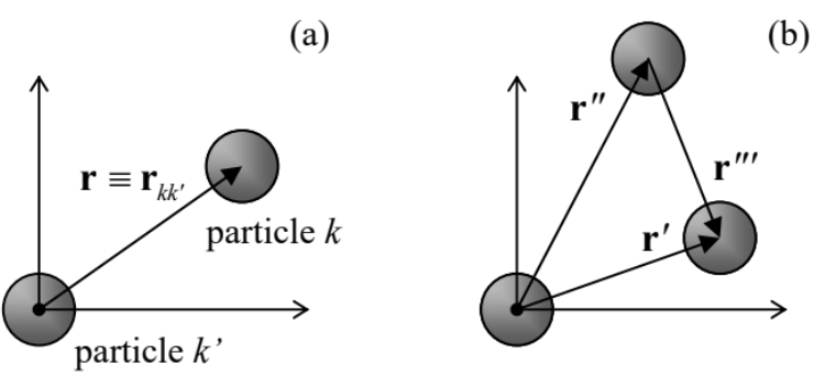
It is convenient to think about the \(\mathbf{r}_{kk'} \equiv \mathbf{r}_k – \mathbf{r}_{k'}\) as the radius-vector of the particle number \(k\) in the reference frame with the origin placed at the center of the particle number \(k'\) – see Figure \(\PageIndex{1a}\).

Figure \(\PageIndex{1}\): The definition of the interparticle distance vectors at their (a) pair and (b) triple interactions.

Then in Equation (\ref{91}), we may first calculate the integral over \(\mathbf{r}_{k'}\), while keeping the distance vector \(\mathbf{r}_{kk'}\), and hence \(U(\mathbf{r}_{kk'}\)), constant, getting one more factor \(V\). Moreover, since all particle pairs are similar, in the remaining integral over \(\mathbf{r}_{kk'}\) we may drop the radius-vector's index, so that Equation (\ref{90}) becomes

\[F = F_{ideal} - \frac{T}{V^N} \frac{N^2}{2} V^{N-1} \int \left(e^{-U(\mathbf{r})/T}-1\right) d^3r \equiv F_{ideal} + \frac{T}{V} N^2 B(T), \label{92}\]

where the function \(B(T)\), called the second virial coefficient,⁴² has an especially simple form for spherically-symmetric interactions:

Second virial coefficient:

\[\boxed{B(T) \equiv \frac{1}{2} \int \left(1-e^{-U(\mathbf{r})/T}\right) d^3r \rightarrow \frac{1}{2} \int^{\infty}_0 4\pi r^2 dr \left(1-e^{-U(r)/T}\right). } \label{93}\]

From Equation (\ref{92}), and the second of the thermodynamic relations (\(1.4.12\)), we already know something particular about the equation of state \(P(V, T)\):

\[P = -\left(\frac{\partial F}{\partial V}\right)_{T,N} = P_{ideal} + \frac{N^2T}{V^2} B(T) = T\left[ \frac{N}{V} + B(T) \frac{N^2}{V^2}\right]. \label{94}\]

We see that at a fixed gas density \(n = N/V\), the pair interaction creates additional pressure, proportional to \((N/V)^2 = n^2\) and a function of temperature, \(B(T)T\).

Let us calculate \(B(T)\) for a few simple models of particle interactions. The solid curve in Figure \(\PageIndex{2}\) shows (schematically) a typical form of the interaction potential between electrically neutral atoms/molecules. At large distances the interaction of particles that do not their own permanent electrical dipole moment \(\mathbf{p}\), is dominated by the attraction (the so-called London dispersion force) between the correlated components of the spontaneously induced dipole moments, giving \(U(r) \rightarrow r^{-6}\) at \(r \rightarrow \infty \).⁴³ At closer distances the potential is repulsive, growing very fast at \(r \rightarrow 0\), but its quantitative form is specific for particular atoms/molecules.⁴⁴ The crudest description of such repulsion is given by the so-called hardball model:

\[U(r)= \begin{cases} +\infty, & \text{ for } 0 < r < 2r_0, \\ 0, & \text{ for } 2r_0 <r<\infty , \end{cases} \label{95}\]

– see the dashed line and the inset in Figure \(\PageIndex{2}\).

Figure \(\PageIndex{2}\): Pair interactions of particles. Solid line: a typical interaction potential; dashed line: its hardball model (\ref{95}); dash-dotted line: the improved model (\ref{97}) – all schematically. The inset illustrates the hardball model’s physics.

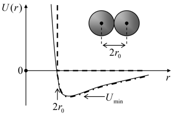
As Equation (\ref{93}) shows, in this model the second virial coefficient is temperature-independent:

\[B(T) = b \equiv \frac{1}{2} \int^{2r_0}_0 4\pi r^2 dr = \frac{2\pi}{3} ( 2r_0)^3 \equiv 4V_0, \quad \text{ where } V_0 \equiv \frac{4\pi}{3} r_0^3, \label{96}\]

so that the equation of state (\ref{94}) still gives a linear dependence of pressure on temperature.

\[U(r)= \begin{cases} +\infty, && \text{ for } 0 < r < 2r_0, \\ U(r), & \text{ with } |U|<<T, & \text{ for } 2r_0 <r<\infty . \end{cases} \label{97}\]

For this improved model, Equation (\ref{93}) yields:

\[B(T)=b+\frac{1}{2} \int^{\infty}_{2r_0} 4\pi r^2 dr \frac{U(r)}{T} \equiv b - \frac{a}{T}, \quad \text{ with } a \equiv 2\pi \int^{\infty}_{2r_0} r^2 dr|U(r)|. \label{98}\]

In this model, the equation of state (\ref{94}) acquires a temperature-independent term:

\[P = T \left[ \frac{N}{V}+\left(\frac{N}{V}\right)^2 \left(b-\frac{a}{T}\right)\right] \equiv T \left[ \frac{N}{V} + b\left(\frac{N}{V}\right)^2\right] - a\left(\frac{N}{V}\right)^2. \label{99}\]

Still, the correction to the ideal-gas pressure is proportional to \((N/V)^2\) and has to be relatively small for this result to be valid.

Generally, the right-hand side of Equation (\ref{99}) may be considered as the sum of two leading terms in the general expansion of \(P\) into the Taylor series in the density \(n = N/V\) of the gas:

Pressure: virial expansion

\[\boxed{P = T \left[ \frac{N}{V}+B(T)\left(\frac{N}{V}\right)^2 +C(T) \left(\frac{N}{V}\right)^3 +...\right], } \label{100}\]

where \(C(T)\) is called the third virial coefficient. It is natural to ask how can we calculate \(C(T)\) and the higher virial coefficients. This may be done, first of all, just by a careful direct analysis of Equation (\ref{90}),⁴⁶ but I would like to use this occasion to demonstrate a different, very interesting and counter-intuitive approach, called the cluster expansion method,⁴⁷ which allows streamlining such calculations.

Let us apply to our system, with the energy given by Equation (\ref{87}), the grand canonical distribution. (Just as in Sec. 2, we may argue that if the average number \(\langle N\rangle\) of particles in a member of a grand canonical ensemble, with fixed \(\mu\) and \(T\), is much larger than 1, the relative fluctuations of \(N\) are small, so that all its thermodynamic properties should be similar to those when \(N\) is exactly fixed.) For our current case, Equation (\(2.7.8\)) takes the form

\[\Omega = -T \ln \sum^{\infty}_{N=0} Z_N, \quad \text{ with } Z_N \equiv e^{\mu N/t} \sum_m e^{-E_{m,N}/T}, E_{m,N} = \sum^N_{k=1} \frac{p_k^2}{2m} + U (r_1,...,r_N). \label{101}\]

(Notice that here, as at all discussions of the grand canonical distribution, \(N\) means a particular rather than the average number of particles.) Now let us try to forget for a minute that in real systems of interest the number of particles is extremely large, and start to calculate, one by one, the first terms \(Z_N\).

In the term with \(N = 0\), both contributions to \(E_{m,N}\) vanish, and so does the factor \(\mu N/T\), so that \(Z_0 = 1\). In the next term, with \(N = 1\), the interaction term vanishes, so that \(E_{m,1}\) is reduced to the kinetic energy of one particle, giving

\[Z_1 = e^{\mu /T} \sum_k \text{exp}\left\{-\frac{p_k^2}{2mT}\right\}.\label{102}\]

Making the usual transition from the summation to integration, we may write

\[Z_1 = ZI_1, \text{ where } Z \equiv e^{u/T} \frac{gV}{(2 \pi \hbar )^3} \int \text{exp} \left\{-\frac{p^2}{2mT}\right\} d^3p, \text{ and } I_1 \equiv 1. \label{103}\]

This is the same simple (Gaussian) integral as in Equation (\(3.1.6\)), giving

\[Z = e^{\mu / T} \frac{gV}{(2\pi \hbar )^3 } ( 2 \pi m T)^{3/2} = e^{\mu / T} gV \left( \frac{mT}{2\pi \hbar^2} \right)^{3/2}.\label{104}\]

Now let us explore the next term, with \(N = 2\), which describes, in particular, pair interactions \(U = U(\mathbf{r})\), with \(\mathbf{r} = \mathbf{r} – \mathbf{r}'\). Due to the assumed particle indistinguishability, this term needs the “correct Boltzmann counting" factor 1/2! – cf. Eqs. (\(3.1.12\)) and (\ref{88}):

\[Z_2 = e^{2\mu / T} \frac{1}{2!} \sum_{k,k'} \left[ \text{exp}\left\{-\frac{p^2_k}{2mT}-\frac{p^2_{k'}}{2mT}\right\}e^{-U(\mathbf{r})/T}\right]. \label{105}\]

Since \(U\) is coordinate-dependent, here the transfer from the summation to integration should be done more carefully than in the first term – cf. Eqs. (\(3.1.25\)) and (\ref{88}):

\[Z_2 = e^{2\mu / T} \frac{1}{2!} \frac{(gV)^2}{(2\pi \hbar )^6} \int \text{exp} \left\{-\frac{p^2}{2mT}\right\}d^3 p \times \int \text{exp}\left\{-\frac{p^{'2}}{2mT}\right\}d^3p'\times \frac{1}{V} \int e^{-U(\mathbf{r})/T} d^3r. \label{106}\]

Comparing this expression with the Equation (\ref{104}) for the parameter \(Z\), we get

\[Z_2 = \frac{Z^2}{2!} I_2, \quad \text{ where } I_2 \equiv \frac{1}{V} \int e^{-U(\mathbf{r})/T} d^3r. \label{107}\]

Acting absolutely similarly, for the third term of the grand canonical sum we may get

\[Z_3 = \frac{Z^3}{3!} I_3, \quad \text{ where } I_3 \equiv \frac{1}{V^2} \int e^{-U(\mathbf{r},\mathbf{r}'')/T} d^3r'd^3r'', \label{108}\]

where \(\mathbf{r}'\) and \(\mathbf{r}"\) are the vectors characterizing the mutual positions of 3 particles – see Figure \(\PageIndex{1b}\).

These results may be extended by induction to an arbitrary \(N\). Plugging the expression for \(Z_N\) into the first of Eqs. (\ref{101}) and recalling that \(\Omega = –PV\), we get the equation of state of the gas in the form

\[P=\frac{T}{V} \ln \left( 1 + ZI_l + \frac{Z^2}{2!} I_2 + \frac{Z^3}{3!} I_3 +...\right). \label{109}\]

As a sanity check: at \(U = 0\), all integrals \(I_N\) are equal to 1, and the expression under the logarithm in just the Taylor expansion of the function \(e^Z\), giving \(P = TZ/V\), and \(\Omega = –PV = –TZ\). In this case, according to the last of Eqs. (\(1.5.13\)), the average number of particles of particles in the system is \(\langle N\rangle = –(\partial \Omega /\partial \mu )_{T,V} = Z\), because since \(Z \propto \text{exp}\{\mu /T\}\), \(\partial Z/\partial \mu = Z/T\).⁴⁸ Thus, in this limit, we have happily recovered the equation of state of the ideal gas.

Returning to the general case of non-zero interactions, let us assume that the logarithm in Equation (\ref{109}) may be also represented as a direct Taylor expansion in \(Z\):

Cluster expansion: pressure

\[\boxed{P=\frac{T}{V} \sum^{\infty}_{l=1} \frac{J_l}{l!} Z^l.}\label{110}\]

(The lower limit of the sum reflects the fact that according to Equation (\ref{109}), at \(Z = 0\), \(P = (T/V) \ln 1 = 0\), so that the coefficient \(J_0\) in a more complete version of Equation (\ref{110}) would equal 0 anyway.) According to Eq, (\(1.5.11\)), this expansion corresponds to the grand potential

\[\Omega = -PV = - T \sum^{\infty}_{l=1} \frac{J_l}{l!} Z^l. \label{111}\]

Again using the last of Eqs. (\(1.5.13\)), and the definition (\ref{104}) of the parameter \(Z\), we get

Cluster expansion: \(\mathbf{\langle N \rangle}\)

\[\boxed{\langle N \rangle = \sum^{\infty}_{l=1} \frac{J_l}{(l-1)!}Z^l.}\label{112}\]

\[\ln (1+\xi ) = \sum^{\infty}_{l=1} (-1)^{l+1} \frac{\xi^l}{l}.\label{113}\]

Using it together with Equation (\ref{109}), we get a Taylor series in \(Z\), starting as

\[P=\frac{T}{V}\left[Z+\frac{Z^2}{2!} (I_2-1)+\frac{Z^3}{3!} [(l_3-1)-3(l_2-1)]+...\right].\label{114}\]

Comparing this expression with Equation (\ref{110}), we see that

\[\begin{align} J_{1} &=1, \nonumber\\ J_{2} &=I_{2}-1=\frac{1}{V} \int\left(e^{-U(\mathbf{r}) / T}-1\right) d^{3} r, \nonumber\\ J_{3} &=\left(I_{3}-1\right)-3\left(I_{2}-1\right) \nonumber\\ &=\frac{1}{V^{2}} \int\left(e^{-U\left(\mathbf{r}^{\prime}, \mathbf{r}^{\prime \prime}\right) / T}-e^{-U(\mathbf{r}) / T}-e^{-U\left(\mathbf{r}^{\prime \prime}\right) / T}-e^{-U\left(\mathbf{r}^{\prime \prime}\right) / T}+2\right) d^{3} r^{\prime} d^{3} r^{\prime \prime}, \ldots \label{115} \end{align} \]

where \(\mathbf{r}''' \equiv \mathbf{r}' − \mathbf{r}"\) - see Figure \(\PageIndex{1b}\). The expression of \(J_2\), describing the pair interactions of particles, is (besides a different numerical factor) equal to the second virial coefficient \(B(T)\) – see Equation (\ref{93}). As a reminder, the subtraction of 1 from the integral \(I_2\) in the second of Eqs. (\ref{115}) makes the contribution of each elementary 3D volume \(d^3r\) into the integral \(J_2\) different from zero only if at this \(\mathbf{r}\) two particles interact \((U \neq 0)\). Very similarly, in the last of Eqs. (\ref{115}), the subtraction of three pair-interaction terms from \((I_3 – 1)\) makes the contribution from an elementary 6D volume \(d^3r'd^3r"\) into the integral \(J_3\) different from zero only if at that mutual location of particles, all three of them interact simultaneously, etc.

In order to illustrate the cluster expansion method at work, let us eliminate the factor \(Z\) from the system of equations (\ref{110}) and (\ref{112}), with accuracy to terms \(O(Z^2)\). For that, let us spell out these equations up to the terms \(O(Z^3)\):

\[\frac{PV}{T} = J_1Z+\frac{J_2}{2}Z^2+\frac{J_3}{6}Z^3+...,\label{116}\]

\[\langle N \rangle = J_1Z + J_2 Z^2 + \frac{J_3}{2}Z^3+...,\label{117}\]

and then divide these two expressions. We get the following result:

\[\frac{PV}{\langle N \rangle T} = \frac{1 + (J_2 / 2J_1 ) Z + (J_3 / 6 J_1) Z^2 +...}{1+(J_2/J_1)Z + (J_3 / 2J_1 )Z^2+...} \approx 1 - \frac{J_2}{2J_1} Z + \left(\frac{J^2_2}{2J^2_1} - \frac{J_3}{3J_1}\right)Z^2,\label{118}\]

whose final form is accurate to terms \(O(Z^2)\). In this approximation, we may again use Equation (\ref{117}), now solved for \(Z\) with the same accuracy:

\[Z \approx \langle N \rangle - \frac{J_2}{J_1} \langle N \rangle^2.\label{119}\]

Plugging this expression into Equation (\ref{118}), we get the virial expansion (\ref{100}) with

\(\mathbf{2^{nd}}\) and \(\mathbf{3^{rd}}\) virial coefficients:

\[\boxed{ B(T) = - \frac{J_2}{2J_1} V, \quad C(T) = \left(\frac{J_2^2}{J^2_1}-\frac{J_3}{3J_1}\right) V^2. } \label{120}\]

The first of these relations, combined with the first two of Eqs. (\ref{115}), yields for the \(2^{nd}\) virial coefficient the same Equation (\ref{96}), \(B(T) = 4V_0\), that was obtained from the Gibbs distribution. The second of these relations enables the calculation of the \(3^{rd}\) virial coefficient \(C(T)\). (Let me leave the calculation of \(J_3\) and \(C(T)\), for the hardball model, for the reader's exercise.) Evidently, a more complete solution of Eqs. (\ref{114}), (\ref{116}), and (\ref{117}) may be used to calculate an arbitrary virial coefficient, though starting from the \(5^{th}\) coefficient, such calculations may be completed only numerically even in the simplest hardball model.