
4.5: Ising model - Exact and numerical results


- Last updated
- Sep 20, 2022
- Save as PDF

( \newcommand{\kernel}{\mathrm{null}\,}\)
In order to evaluate the main prediction (4.4.14) of the Weiss theory, let us now discuss the exact (analytical) and quasi-exact (numerical) results obtained for the Ising model, going from the lowest value of dimensionality, d=0, to its higher values. Zero dimensionality means that the spin has no nearest neighbors at all, so that the first term of Equation (4.2.3) vanishes. Hence Equation (4.4.6) is exact, with hef=h, and so is its solution (4.4.11). Now we can simply use Equation (4.4.18), with J=0, i.e. Tc=0, reducing this result to the so-called Curie law:
Curie law:
χ=1T.
It shows that the system is paramagnetic at any temperature. One may say that for d=0 the Weiss molecular-field theory is exact – or even trivial. (However, in some sense it is more general than the Ising model, because as we know from Chapter 2, it gives the exact result for a fully quantum mechanical treatment of any two-level system, including spin-1/2.) Experimentally, the Curie law is approximately valid for many so-called paramagnetic materials, i.e. 3D systems with sufficiently weak interaction between particle spins.
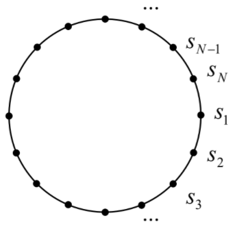
The case d=1 is more complex but has an exact analytical solution. A simple (though not the simplest!) way to obtain it is to use the so-called transfer matrix approach.40 For this, first of all, we may argue that most properties of a 1D system of N>>1 spins (say, put at equal distances on a straight line) should not change noticeably if we bend that line gently into a closed ring (Figure 4.5.1), assuming that spins s1 and sN interact exactly as all other next-neighbor pairs. Then the energy (4.2.3) becomes
Em=−(Js1s2+Js2s3+...+JsNs1)−(hs1+hs2+...+hsN).
Let us regroup the terms of this sum in the following way:
Em=−[(h2s1+Js1s2+h2s2)+(h2s2+Js2s3+h2s3)+…+(h2sN+JNs1+h2s1)],
so that the group inside each pair of parentheses depends only on the state of two adjacent spins. The corresponding statistical sum,
Z=∑sk=±1,fkrk=1,2,…Nexp{hs12T+Js1s2T+hs22T}exp{hs22T+Js2s3T+hs32T}…exp{hsN2T+JsNs1T+hs12T},
still has 2N terms, each corresponding to a certain combination of signs of N spins. However, each operand of the product under the sum may take only four values, corresponding to four different combinations of its two arguments:
exp{hsk2T+Jsksk+1T+hsk+12T}={exp{(J+h)/T}, for sk=sk+1=+1,exp{(J−h)/T}, for sk=sk+1=−1,exp{−J/T}, for sk=−sk+1=±1.
M≡(exp{(J+h)/T}exp{−J/T}exp{−J/T}exp{(J−h)/T}),
so that the whole statistical sum (???) may be recast as a product:
Z=∑jk=1,2Mj1j2Mj2j3…MjN−1jNMjNj1.
According to the basic rule of matrix multiplication, this sum is just
Z=Tr(MN).
Linear algebra tells us that this trace may be represented just as
Z=λN++λN−,
where λ± are the eigenvalues of the transfer matrix M, i.e. the roots of its characteristic equation,
|exp{(J+h)/T}−λexp{−J/T}exp{−J/T}exp{(J−h)/T}−λ|=0.
A straightforward calculation yields
λ±=exp{JT}[coshhT±(sinh2hT+exp{−4JT})1/2].
The last simplification comes from the condition N>>1 – which we need anyway, to make the ring model sufficiently close to the infinite linear 1D system. In this limit, even a small difference of the exponents, λ+>λ−, makes the second term in Equation (???) negligible, so that we finally get
Z=λN+=exp{NJT}[coshhT+(sinh2hT+exp{−4JT})1/2]N.
From here, we can find the free energy per particle:
FN=TNln1Z=−J−Tln[coshhT+(sinh2hT+exp{−4JT})1/2],
and then use thermodynamics to calculate such variables as entropy – see the first of Eqs. (1.4.12).
However, we are mostly interested in the order parameter defined by Equation (4.2.5): η≡⟨sj⟩. The conceptually simplest approach to the calculation of this statistical average would be to use the sum (2.1.7), with the Gibbs probabilities Wm=Z−1exp{−Em/T}. However, the number of terms in this sum is 2N, so that for N>>1 this approach is completely impracticable. Here the analogy between the canonical pair {–P,V} and other generalized force-coordinate pairs {F,q}, in particular {μ0H(rk),mk} for the magnetic field, discussed in Secs. 1.1 and 1.4, becomes invaluable – see in particular Equation (1.1.5). (In our normalization (4.2.2), and for a uniform field, the pair {μ0H(rk),mk} becomes {h,sk}.) Indeed, in this analogy the last term of Equation (4.2.3), i.e. the sum of N products (–hsk) for all spins, with the statistical average (–Nhη), is similar to the product PV, i.e. the difference between the thermodynamic potentials F and G≡F+PV in the usual “P−V thermodynamics”. Hence, the free energy F given by Equation (???) may be understood as the Gibbs energy of the Ising system in the external field, and the equilibrium value of the order parameter may be found from the last of Eqs. (1.4.16) with the replacements –P→h,V→Nη:
Nη=−(∂F∂h)T, i.e.η=−[∂(F/N)∂h]T.
Note that this formula is valid for any model of ferromagnetism, of any dimensionality, if it has the same form of interaction with the external field as the Ising model.
For the 1D Ising ring with N>>1, Eqs. (???) and (???) yield
η=sinhhT/(sinh2hT+exp{−4JT})1/2, giving χ≡∂η∂h|h=0=1Texp{2JT}.
This result means that the 1D Ising model does not exhibit a phase transition, i.e., in this model Tc=0. However, its susceptibility grows, at T→0, much faster than the Curie law (???). This gives us a hint that at low temperatures the system is “virtually ferromagnetic”, i.e. has the ferromagnetic order with some rare random violations. (Such violations are commonly called low-temperature excitations.) This interpretation may be confirmed by the following approximate calculation. It is almost evident that the lowest-energy excitation of the ferromagnetic state of an open-end 1D Ising chain at h=0 is the reversal of signs of all spins in one of its parts – see Figure 4.5.2.
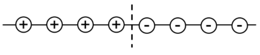
Indeed, such an excitation (called the Bloch wall42) involves the change of sign of just one product sksk′, so that according to Equation (4.2.3), its energy EW (defined as the difference between the values of Em with and without the excitation) equals 2J, regardless of the wall's position.43 Since in the ferromagnetic Ising model, the parameter J is positive, EW>0. If the system “tried” to minimize its internal energy, having any wall in the system would be energy-disadvantageous. However, thermodynamics tells us that at T≠0, the system's thermal equilibrium corresponds to the minimum of the free energy F≡E–TS, rather than just energy E.44 Hence, we have to calculate the Bloch wall's contribution FW to the free energy. Since in an open-end linear chain of N>>1 spins, the wall can take (N–1)≈N positions with the same energy EW, we may claim that the entropy SW associated with this excitation is lnN, so that
FW≡EW−TSW≈2J−TlnN.
This result tells us that in the limit N→∞, and at T≠0, walls are always free-energy-beneficial, thus explaining the absence of the perfect ferromagnetic order in the 1D Ising system. Note, however, that since the logarithmic function changes extremely slowly at large values of its argument, one may argue that a large but finite 1D system should still feature a quasi-critical temperature
"T_c" = \frac{2J}{\ln N}, \label{93}
below which it would be in a virtually complete ferromagnetic order. (The exponentially large susceptibility (\ref{91}) is another manifestation of this fact.)
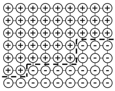
Now let us apply a similar approach to estimate T_c of a 2D Ising model, with open borders. Here the Bloch wall is a line of a certain total length L – see Figure \PageIndex{3}. (For the example presented in that figure, counting from the left to the right, L = 2 + 1 + 4 + 2 + 3 = 12 lattice periods.) Evidently, the additional energy associated with such a wall is E_W = 2JL, while the wall's entropy S_W may be estimated using the following reasoning. Let the wall be formed along the path of a “Manhattan pedestrian” traveling between its nodes. (The dashed line in Figure \PageIndex{3} is an example of such a path.) At each junction, the pedestrian may select 3 choices of 4 possible directions (except the one that leads backward), so that there are approximately 3^{(L-1)} \approx 3^L options for a walk starting from a certain point. Now taking into account that the open borders of a square-shaped lattice with N spins have a length of the order of N^{1/2}, and the Bloch wall may start from any of them, there are approximately M \sim N^{1/2}3^L different walks between two borders. Again estimating S_W as \ln M, we get
F_W = E_W - TS_W \approx 2JL - T \ln (N^{1/2}3^L) \equiv L (2J - T \ln 3 ) - (T / 2) \ln N. \label{94}
(Actually, since L scales as N^{1/2} or higher, at N \rightarrow \infty the last term in Equation (\ref{94}) is negligible.) We see that the sign of the derivative \partial F_W /\partial L depends on whether the temperature is higher or lower than the following critical value:
T_c = \frac{2J}{\ln 3} \approx 1.82 \ J. \label{95}
At T < T_c, the free energy's minimum corresponds to L \rightarrow 0, i.e. the Bloch walls are free-energy detrimental, and the system is in the purely ferromagnetic phase.
So, for d = 2 the estimates predict a non-zero critical temperature of the same order as the Weiss theory (according to Equation (4.4.14), in this case T_c = 4J). The major approximation implied in our calculation leading to Equation (\ref{95}) is disregarding possible self-crossings of the “Manhattan walk”. The accurate counting of such self-crossings is rather difficult. It had been carried out in 1944 by L. Onsager; since then his calculations have been redone in several easier ways, but even they are rather cumbersome, and I will not have time to discuss them.45 The final result, however, is surprisingly simple:
Onsager's exact result:
\boxed{ T_c = \frac{2J}{\ln(1+\sqrt{2})} \approx 2.269 \ J,} \label{96}
i.e. showing that the simple estimate (\ref{95}) is off the mark by only \sim 20%.
The Onsager solution, as well as all alternative solutions of the problem that were found later, are so “artificial” (2D-specific) that they do not give a clear way towards their generalization to other (higher) dimensions. As a result, the 3D Ising problem is still unsolved analytically. Nevertheless, we do know T_c for it with extremely high precision – at least to the 6^{th} decimal place. This has been achieved by numerical methods; they deserve a thorough discussion because of their importance for the solution of other similar problems as well.
Conceptually, this task is rather simple: just compute, to the desired precision, the statistical sum of the system (4.2.3):
Z =\sum_{s_{k}=\pm 1, for \atop k=1,2, \ldots N} \exp \left\{\frac{J}{T} \sum_{\{k,k'\}} s_{k}s_{k'} + \frac{h}{T} \sum_k s_k \right\}.\label{97}
As soon as this has been done for a sufficient number of values of the dimensionless parameters J/T and h/T, everything becomes easy; in particular, we can compute the dimensionless function
F /T = −\ln Z , \label{98}
and then find the ratio J/T_c as the smallest value of the parameter J/T at that the ratio F/T (as a function of h/T) has a minimum at zero field. However, for any system of a reasonable size N, the “exact” computation of the statistical sum (\ref{97}) is impossible, because it contains too many terms for any supercomputer to handle. For example, let us take a relatively small 3D lattice with N = 10 \times 10 \times 10 = 10^3 spins, which still feature substantial boundary artifacts even using the periodic boundary conditions, so that its phase transition is smeared about T_c by \sim 3%. Still, even for such a crude model, Z would include 2^{1,000} \equiv (2^{10})^{100} \approx (10^3)^{100} \equiv 10^{300} terms. Let us suppose we are using a modern exaflops-scale supercomputer performing 10^{18} floating-point operations per second, i.e. \sim 10^{26} such operations per year. With those resources, the computation of just one statistical sum would require \sim 10^{(300-26)} = 10^{274} years. To call such a number “astronomic” would be a strong understatement. (As a reminder, the age of our Universe is close to 1.3 \times 10^{10} years – a very humble number in comparison.)
This situation may be improved dramatically by noticing that any statistical sum,
Z = \sum_m \exp \left\{ - \frac{E_m}{T}\right\}, \label{99}
is dominated by terms with lower values of E_m. To find those lowest-energy states, we may use the following powerful approach (belonging to a broad class of numerical Monte-Carlo techniques), which essentially mimics one (randomly selected) path of the system's evolution in time. One could argue that for that we would need to know the exact laws of evolution of statistical systems,46 that may differ from one system to another, even if their energy spectra E_m are the same. This is true, but since the genuine value of Z should be independent of these details, it may be evaluated using any reasonable kinetic model that satisfies certain general rules. In order to reveal these rules, let us start from a system with just two states, with energies E_m and E_{m'} = E_m + \Delta – see Figure \PageIndex{4}.
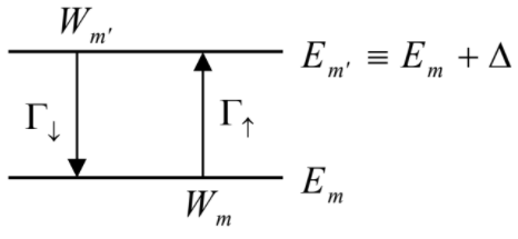
In the absence of quantum coherence between the states (see Sec. 2.1), the equations for the time evolution of the corresponding probabilities W_m and W_{m'} should depend only on the probabilities (plus certain constant coefficients). Moreover, since the equations of quantum mechanics are linear, these master equations should be also linear. Hence, it is natural to expect them to have the following form,
Master equations:
\boxed{ \frac{dW_m}{dt} = W_{m'} \Gamma_{\downarrow} - W_m \Gamma_{\uparrow}, \quad \frac{dW_{m'}}{dt} = W_m \Gamma_{\uparrow} - W_{m'} \Gamma_{\downarrow}, } \label{100}
where the coefficients \Gamma_{\uparrow} and \Gamma_{\downarrow} have the physical sense of the rates of the corresponding transitions (see Figure \PageIndex{4}); for example, \Gamma_{\uparrow} dt is the probability of the system's transition into the state m' during an infinitesimal time interval dt, provided that at the beginning of that interval it was in the state m with full certainty: W_m = 1, W_{m'} = 0.47 Since for the system with just two energy levels, the time derivatives of the probabilities have to be equal and opposite, Eqs. (\ref{100}) describe an (irreversible) redistribution of the probabilities while keeping their sum W = W_m + W_{m'} constant. According to Eqs. (\ref{100}), at t \rightarrow \infty the probabilities settle to their stationary values related as
\frac{W_{m'}}{W_m} = \frac{\Gamma_{\uparrow}}{\Gamma_{\downarrow}}. \label{101}
Now let us require these stationary values to obey the Gibbs distribution (2.4.7); from it
\frac{W_{m'}}{W_m} = \exp \left\{ \frac{E_m - E_{m'}}{T}\right\} = \exp \left\{-\frac{\Delta}{T}\right\} < 1. \label{102}
Comparing these two expressions, we see that the rates have to satisfy the following detailed balance relation:
Detailed balance:
\boxed{ \frac{\Gamma_{\uparrow}}{\Gamma_{\downarrow}} =\exp \left\{-\frac{\Delta}{T}\right\} .} \label{103}
Now comes the final step: since the rates of transition between two particular states should not depend on other states and their occupation, Equation (\ref{103}) has to be valid for each pair of states of any multi-state system. (By the way, this relation may serve as an important sanity check: the rates calculated using any reasonable model of a quantum system have to satisfy it.)
The detailed balance yields only one equation for two rates \Gamma_{\uparrow} and \Gamma_{\downarrow}; if our only goal is the calculation of Z, the choice of the other equation is not too important. A very simple choice is
\Gamma (\Delta) \propto \gamma (\Delta ) \equiv \begin{cases} 1, && \text{ if } \Delta < 0, \\ \exp \{-\Delta / T\}, && \text{ otherwise,} \end{cases} \label{104}
where \Delta is the energy change resulting from the transition. This model, which evidently satisfies the detailed balance relation (\ref{103}), is very popular (despite the unphysical cusp this function has at \Delta = 0), because it enables the following simple Metropolis algorithm (Figure \PageIndex{5}).
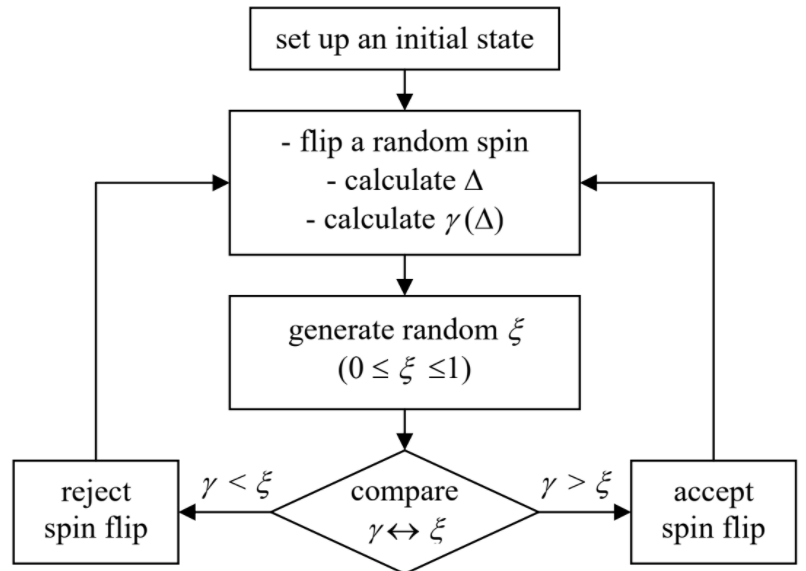
The calculation starts by setting a certain initial state of the system. At relatively high temperatures, the state may be generated randomly; for example, in the Ising system, the initial state of each spin s_k may be selected independently, with a 50% probability. At low temperatures, starting the calculations from the lowest-energy state (in particular, for the Ising model, from the ferromagnetic state s_k = \text{sgn}(h) = const) may give the fastest convergence. Now one spin is flipped at random, the corresponding change \Delta of the energy is calculated,48 and plugged into Equation (\ref{104}) to calculate \gamma (\Delta ). Next, a pseudo-random number generator is used to generate a random number \xi , with the probability density being constant on the segment [0, 1]. (Such functions are available in virtually any numerical library.) If the resulting \xi is less than \gamma (\Delta ), the transition is accepted, while if \xi > \gamma (\Delta ), it is rejected. Physically, this means that any transition down the energy spectrum (\Delta < 0) is always accepted, while those up the energy profile (\Delta > 0) are accepted with the probability proportional to \exp\{–\Delta /T\}.49 After sufficiently many such steps, the statistical sum (\ref{99}) may be calculated approximately as a partial sum over the states passed by the system. (It may be better to discard the contributions from a few first steps, to avoid the effects of the initial state choice.)
This algorithm is extremely efficient. Even with modest computers available in the 1980s, it has allowed simulating a 3D Ising system of (128)^3 spins to get the following result: J/T_c \approx 0.221650 \pm 0.000005. For all practical purposes, this result is exact – so that perhaps the largest benefit of the possible future analytical solution of the infinite 3D Ising problem will be a virtually certain Nobel Prize for its author. Table \PageIndex{1} summarizes the values of T_c for the Ising model. Very visible is the fast improvement of the prediction accuracy of the molecular-field theory – which is asymptotically correct at d \rightarrow \infty .
Table \PageIndex{1}: The critical temperature T_c (in the units of J) of the Ising model of a ferromagnet (J > 0), for several values of dimensionality d
|
d |
Molecular-field theory – Equation (4.4.14) |
Exact value |
Exact value's source |
|
0 |
0 |
0 |
Gibbs distribution |
|
1 |
2 |
0 |
Transfer matrix theory |
|
2 |
4 |
2.269... |
Onsager's solution |
|
3 |
6 |
4.513... |
Numerical simulation |
Finally, I need to mention the renormalization-group (“RG”) approach,50 despite its low efficiency for the Ising-type problems. The basic idea of this approach stems from the scaling law (4.2.10)- (4.2.11): at T = T_c the correlation radius r_c diverges. Hence, the critical temperature may be found from the requirement for the system to be spatially self-similar. Namely, let us form larger and larger groups (“blocks”) of adjacent spins, and require that all properties of the resulting system of the blocks approach those of the initial system, as T approaches T_c.
Let us see how this idea works for the simplest nontrivial (1D) case, described by the statistical sum (\ref{80}). Assuming N to be even (which does not matter at N \rightarrow \infty ), and adding an inconsequential constant C to each exponent (for the purpose that will be clear soon), we may rewrite this expression as
Z=\sum_{s_{k}=\pm 1} \prod_{k=1,2, \ldots_{N}} \exp \left\{\frac{h}{2 T} s_{k}+\frac{J}{T} s_{k} s_{k+1}+\frac{h}{2 T} s_{k+1}+C\right\} . \label{105}
Let us group each pair of adjacent exponents to recast this expression as a product over only even numbers k,
Z=\sum_{s_{k}=\pm 1} \prod_{k=2,4, \ldots N} \exp \left\{\frac{h}{2 T} s_{k-1}+s_{k}\left[\frac{J}{T}\left(s_{k-1}+s_{k+1}\right)+\frac{h}{T}\right]+\frac{h}{2 T} s_{k+1}+2 C\right\}, \label{106}
and carry out the summation over two possible states of the internal spin s_k explicitly:
\begin{align} Z &=\sum_{s_{k}=\pm 1} \prod_{k=2,4, \ldots N}\left[\begin{array}{c} \exp \left\{\frac{h}{2 T} s_{k-1}+\frac{J}{T}\left(s_{k-1}+s_{k+1}\right)+\frac{h}{T}+\frac{h}{2 T} s_{k+1}+2 C\right\} \\ +\exp \left\{\frac{h}{2 T} s_{k-1}-\frac{J}{T}\left(s_{k-1}+s_{k+1}\right)-\frac{h}{T}+\frac{h}{2 T} s_{k+1}+2 C\right\} \end{array}\right] \nonumber\\ & \equiv \sum_{s_{i}=+1} \prod_{k=2.4, \ldots N} 2 \cosh \left\{\frac{J}{T}\left(s_{k-1}+s_{k+1}\right)+\frac{h}{T}\right\} \exp \left\{\frac{h}{2 T}\left(s_{k-1}+s_{k+1}\right)+2 C\right\}. \label{107}\end{align}
Now let us require this statistical sum (and hence all statistical properties of the system of 2-spin blocks) to be identical to that of the Ising system of N/2 spins, numbered by odd k:
Z^{\prime}=\sum_{s_{k}=1} \prod_{k=2,4, \ldots, N} \exp \left\{\frac{J^{\prime}}{T} s_{k-1} s_{k+1}+\frac{h^{\prime}}{T} s_{k+1}+C^{\prime}\right\}, \label{108}
with some different parameters h', J', and C', for all four possible values of s_{k-1} = \pm 1 and s_{k+1} = \pm 1. Since the right-hand side of Equation (\ref{107}) depends only on the sum (s_{k-1} + s_{k+1}), this requirement yields only three (rather than four) independent equations for finding h', J', and C'. Of them, the equations for h' and J' depend only on h and J (but not on C),51 and may be represented in an especially simple form,
RG equations for 1D Ising model:
\boxed{x^{\prime}=\frac{x(1+y)^{2}}{(x+y)(1+x y)}, \quad y^{\prime}=\frac{y(x+y)}{1+x y}}, \label{109}
if the following notation is used:
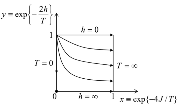
x \equiv \exp \left\{-4 \frac{J}{T}\right\}, \quad y \equiv \exp \left\{-2 \frac{h}{T}\right\}. \label{110}
Now the grouping procedure may be repeated, with the same result (\ref{109})-(\ref{110}). Hence these equations may be considered as recurrence relations describing repeated doubling of the spin block size. Figure \PageIndex{6} shows (schematically) the trajectories of this dynamic system on the phase plane [x, y]. (Each trajectory is defined by the following property: for each of its points \{x, y\}, the point \{x', y'\} defined by the “mapping” Equation (\ref{109}) is also on the same trajectory.) For ferromagnetic coupling (J > 0) and h > 0, we may limit the analysis to the unit square 0 \leq x, y \leq 1. If this flow diagram had a stable fixed point with x' = x = x_{\infty} \neq 0 (i.e. T/J < \infty ) and y' = y = 1 (i.e. h = 0), then the first of Eqs. (\ref{110}) would immediately give us the critical temperature of the phase transition in the field-free system:
T_c = \frac{4J}{\ln (1/x_{\infty})}. \label{111}
However, Figure \PageIndex{6} shows that the only fixed point of the 1D system is x = y = 0, which (at a finite coupling J) should be interpreted as T_c = 0. This is of course in agreement with the exact result of the transfer-matrix analysis, but does not provide any additional information.
Unfortunately, for higher dimensionalities, the renormalization-group approach rapidly becomes rather cumbersome and requires certain approximations, whose accuracy cannot be easily controlled. For the 2D Ising system, such approximations lead to the prediction T_c \approx 2.55 \ J, i.e. to a substantial difference from the exact result (\ref{96}).