4.4: Ising model - Weiss molecular-field theory

The Landau mean-field theory is phenomenological in the sense that even within the range of its validity, it tells us nothing about the value of the critical temperature $T_c$ and other parameters (in Equation ($4.3.6$), the coefficients $a$, $b$, and $c$), so that they have to be found from a particular “microscopic” model of the system under analysis. In this course, we would have time to discuss only the Ising model ($4.2.3$) for various dimensionalities $d$.

$$F = −(NJd )\eta^2 − Nh\eta . \label{59}$$

This energy is plotted in Figure $\PageIndex{1a}$ as a function of $\eta$, for several values of $h$.

Figure $\PageIndex{1}$: Field dependences of (a) the free energy profile and (b) the order parameter (i.e. magnetization) in the crudest mean-field approach to the Ising model.

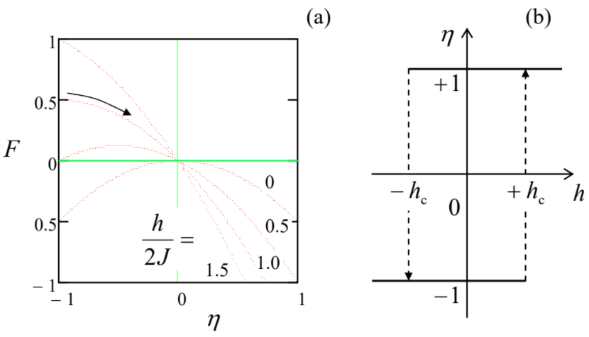
The plots show that at $h = 0$, the system may be in either of two stable states, with $\eta = \pm 1$, corresponding to two different spin directions (i.e. two different directions of magnetization), with equal energy.³⁵ (Formally, the state with $\eta = 0$ is also stationary, because at this point $\partial F/\partial \eta = 0$, but it is unstable, because for the ferromagnetic interaction, $J > 0$, the second derivative $\partial^2 F/\partial \eta^2$ is always negative.)

As the external field is increased, it tilts the potential profile, and finally at the critical field,

$$h = h_c \equiv 2Jd , \label{60}$$

So, this simplest mean-field theory ($\ref{59}$) does give a (crude) description of the ferromagnetic ordering. However, this theory grossly overestimates the stability of these states with respect to thermal fluctuations. Indeed, in this theory, there is no thermally-induced randomness at all, until $T$ becomes comparable with the height of the energy barrier separating two stable states,

$$\Delta F \equiv F(\eta = 0) − F(\eta = \pm 1) = NJd , \label{61}$$

which is proportional to the number of particles. At $N \rightarrow \infty$, this value diverges, and in this sense, the critical temperature is infinite, while numerical experiments and more refined theories of the Ising model show that actually its ferromagnetic phase is suppressed at $T > T_c \sim Jd$ – see below.

The accuracy of this theory may be dramatically improved by even an approximate account for thermally-induced randomness. In this approach (suggested in 1907 by Pierre-Ernest Weiss), called the molecular-field theory,³⁸ random deviations of individual spin values from the lattice average,

$$\tilde{s}_k \equiv s_k - \eta, \quad \text{ with } \eta \equiv \langle s_k \rangle , \label{62}$$

are allowed, but considered small, $| \tilde{s}_k <<\eta$. This assumption allows us, after plugging the resulting expression $s_k = \eta + \tilde{s}_k$ to the first term on the right-hand side of Equation ($4.2.3$),

$$E_{m}=-J \sum_{\{ k, k\}} \left(\eta+\tilde{s}_{k}\right) \left(\eta+ \widetilde{s}_{k^{\prime}}\right)-h \sum_{k} s_{k} \equiv-J \sum_{\left\{k, k^{\prime}\right\}} \left[\eta^{2}+\eta \left(\widetilde{s}_{k} +\widetilde{s}_{k^{\prime}} \right)+\tilde{s}_{k} \widetilde{s}_{k^{\prime}}\right]-h \sum_{k} s_{k}, \label{63}$$

ignore the last term in the square brackets. Making the replacement ($\ref{62}$) in the terms proportional to $\tilde{s}_k$, we may rewrite the result as

$$E_m \approx E_m' \equiv (NJd) \eta^2 - h_{ef} \sum_k s_k , \label{64}$$

where $h_{ef}$ is defined as the sum

$$h_{ef} \equiv h + (2Jd) \eta . \label{65}$$

This sum may be interpreted as the effective external field, which takes into account (besides the genuine external field $h$) the effect that would be exerted on spin $s_k$ by its $2d$ next neighbors if they all had non-fluctuating (but possibly continuous) spin values $s_{k'} = \eta$. Such addition to the external field,

Weiss molecular field:

$$\boxed{ h_{mol} \equiv h_{ef} - h = (2Jd ) \eta , } \label{66}$$

is called the molecular field – giving its name to the Weiss theory.

From the point of view of statistical physics, at fixed parameters of the system (including the order parameter $\eta$), the first term on the right-hand side of Equation ($\ref{64}$) is merely a constant energy offset, and $h_{ef}$ is just another constant, so that

$$E_{m}^{\prime}=\text { const }+\sum_{k} \varepsilon_{k}, \quad \text { with } \varepsilon_{k}=-h_{e f} s_{k} \equiv \begin{cases}-h_{\mathrm{ef}}, & \text { for } s_{k}=+1 \\ +h_{\mathrm{ef}}, & \text { for } s_{k}=-1. \end{cases} \label{67}$$

Such separability of the energy means that in the molecular-field approximation the fluctuations of different spins are independent of each other, and their statistics may be examined individually, using the energy spectrum $\varepsilon_k$. But this is exactly the two-level system that was the subject of Problems 2.2- 2.4. Actually, its statistics is so simple that it is easier to redo this fundamental problem starting from scratch, rather than to use the results of those exercises (which would require changing notation).

Indeed, according to the Gibbs distribution ($2.4.7$)-($2.4.8$), the equilibrium probabilities of the states $s_k = \pm 1$ may be found as

$$W_{\pm}=\frac{1}{Z} e^{\pm h_{e f} / T}, \quad \text { with } Z=\exp \left\{+\frac{h_{\mathrm{ef}}}{T}\right\}+\exp \left\{-\frac{h_{\mathrm{ef}}}{T}\right\} \equiv 2 \cosh \frac{h_{\mathrm{ef}}}{T} . \label{68}$$

From here, we may readily calculate $F = –T \ln Z$ and all other thermodynamic variables, but let us immediately use Equation ($\ref{68}$) to calculate the statistical average of $s_j$, i.e. the order parameter:

$$\eta \equiv \langle s_j \rangle = (+1) W_+ + (-1) W_- = \frac{e^{+h_{ef}/T} e^{-h_{ef}/T}}{2 \cosh (h_{ef}/T)} \equiv \tanh \frac{h_{ef}}{T}. \label{69}$$

Now comes the punch line of the Weiss' approach: plugging this result back into Equation ($\ref{65}$), we may write the condition of self-consistency of the molecular-field theory:

Self-consistency equation:

$$\boxed{h_{ef} - h = 2Jd \tanh \frac{h_{ef}}{T}. } \label{70}$$

This is a transcendental equation, which evades an explicit analytical solution, but whose properties may be readily analyzed by plotting both its sides as functions of the same argument, so that the stationary state(s) of the system corresponds to the intersection point(s) of these plots.

First of all, let us explore the field-free case $(h = 0)$, when $h_{ef} = h_{mol} \equiv 2dJ\eta$, so that Equation ($\ref{70}$) is reduced to

$$\eta = \tanh \left( \frac{2Jd}{T} \eta \right), \label{71}$$

giving one of the patterns sketched in Figure $\PageIndex{2}$, depending on the dimensionless parameter $2Jd/T$.

Figure $\PageIndex{2}$: The ferromagnetic phase transition in Weiss' molecular-field theory: two sides of Equation ($\ref{71}$) sketched as functions of $\eta$ for three different temperatures: above $T_c$ (red), below $T_c$ (blue), and equal to $T_c$ (green).

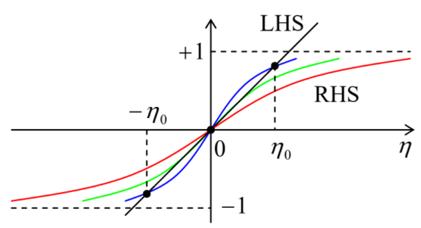
If this parameter is small, the right-hand side of Equation ($\ref{71}$) grows slowly with $\eta$ (see the red line in Figure $\PageIndex{2}$), and there is only one intersection point with the left-hand side plot, at $\eta = 0$. This means that the spin system has no spontaneous magnetization; this is the so-called paramagnetic phase. However, if the parameter $2Jd/T$ exceeds 1, i.e. if $T$ is decreased below the following critical value,

Critical ("Curie") temperature:

$$\boxed{ T_c = 2Jd , } \label{72}$$

the right-hand side of Equation ($\ref{71}$) grows, at small $\eta$, faster than its left-hand side, so that their plots intersect it in 3 points: $\eta = 0$ and $\eta = \pm \eta_0$ – see the blue line in Figure $\PageIndex{2}$. It is almost evident that the former stationary point is unstable, while the two latter points are stable. (This fact may be readily verified by using Equation ($\ref{68}$) to calculate $F$. Now the condition $\partial F/\partial \eta |_{h=0} = 0$ returns us to Equation ($\ref{71}$), while calculating the second derivative, for $T < T_c$ we get $\partial^2 F/\partial \eta^2 > 0$ at $\eta = \pm \eta_0$, and $\partial^2F/\partial \eta^2 < 0$ at $\eta = 0$). Thus, below $T_c$ the system is in the ferromagnetic phase, with one of two possible directions of the average spontaneous magnetization, so that the critical (Curie³⁹) temperature, given by Equation ($\ref{72}$), marks the transition between the paramagnetic and ferromagnetic phases. (Since the stable minimum value of the free energy $F$ is a continuous function of temperature at $T = T_c$, this phase transition is continuous.)

Now let us repeat this graphics analysis to examine how each of these phases responds to an external magnetic field $h \neq 0$. According to Equation ($\ref{70}$), the effect of $h$ is just a horizontal shift of the straight-line plot of its left-hand side – see Figure $\PageIndex{3}$. (Note a different, here more convenient, normalization of both axes.)

Figure $\PageIndex{3}$: External field effects on: (a) a paramagnet $(T > T_c)$, and (b) a ferromagnet $(T < T_c)$.

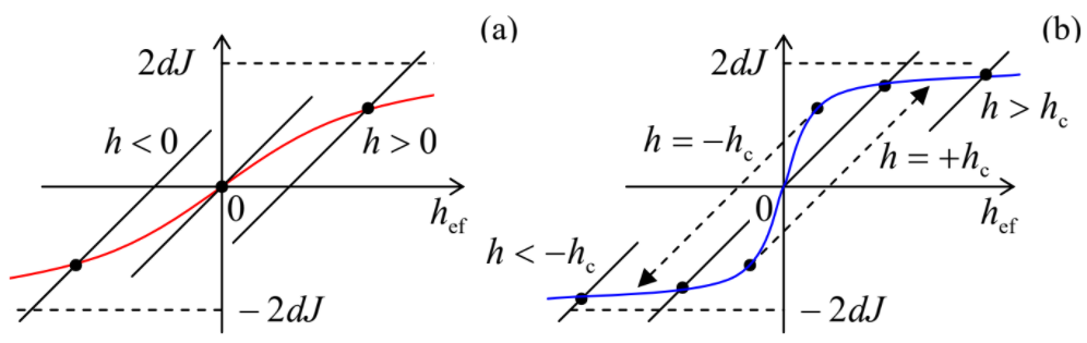
In the paramagnetic case (Figure $\PageIndex{3a}$) the resulting dependence $h_{ef}(h)$ is evidently continuous, but the coupling effect $(J > 0)$ makes it steeper than it would be without spin interaction. This effect may be quantified by the calculation of the low-field susceptibility defined by Equation ($4.2.9$). To calculate it, let us notice that for small $h$, and hence small $h_{ef}$, the function tanh in Equation ($\ref{70}$) is approximately equal to its argument so that Equation ($\ref{70}$) is reduced to

$$h_{ef} - h = \frac{2Jd}{T} h_{ef}, \quad \text{ for } \left| \frac{2Jd}{T} h_{ef} \right| <<1. \label{73}$$

Solving this equation for $h_{ef}$, and then using Equation ($\ref{72}$), we get

$$h_{ef} = \frac{h}{1-2Jd/T} \equiv \frac{h}{1-T_c / T}. \label{74}$$

Recalling Equation ($\ref{66}$), we can rewrite this result for the order parameter:

$$\eta = \frac{h_{ef}-h}{T_c} = \frac{h}{T-T_c}, \label{75}$$

so that the low-field susceptibility

Curie-Weiss law:

$$\boxed{\chi \equiv \left. \frac{\partial \eta}{\partial h} \right|_{h=0} = \frac{1}{T-T_c}, \quad \text{ for } T > T_c. } \label{76}$$

This is the famous Curie-Weiss law, which shows that the susceptibility diverges at the approach to the Curie temperature $T_c$.

In the ferromagnetic case, the graphical solution (Figure $\PageIndex{3b}$) of Equation ($\ref{70}$) gives a qualitatively different result. A field increase leads, depending on the spontaneous magnetization, either to the further saturation of $h_{mol}$ (with the order parameter $\eta$ gradually approaching 1), or, if the initial $\eta$ was negative, to a jump to positive $\eta$ at some critical (coercive) field $h_c$. In contrast with the crude approximation ($\ref{59}$), at $T > 0$ the coercive field is smaller than that given by Equation ($\ref{60}$), and the magnetization saturation is gradual, in a good (semi-qualitative) accordance with experiment.

To summarize, the Weiss molecular-field theory gives an approximate but realistic description of the ferromagnetic and paramagnetic phases in the Ising model, and a very simple prediction ($\ref{72}$) of the temperature of the phase transition between them, for an arbitrary dimensionality $d$ of the cubic lattice. It also enables calculation of other parameters of Landau's mean-field theory for this model – an easy exercise left for the reader. Moreover, the molecular-field approach allows one to obtain analytical (if approximate) results for other models of phase transitions – see, e.g., Problem 18.