6.2: The Ohm law and the Drude formula

Despite its shortcomings, Equation (\(6.1.18\)) is adequate for quite a few applications. Perhaps the most important of them is deriving the Ohm law for dc current in a “nearly-ideal” gas of charged particles, whose only important deviation from ideality is the rare scattering effects described by Equation (\(6.1.17\)). As a result, in equilibrium it is described by the stationary probability \(w_0\) of an ideal gas (see Sec. 3.1):

\[w_0 (\mathbf{r},\mathbf{p},t) = \frac{g}{(2\pi \hbar )^3} \langle N(\varepsilon )\rangle , \label{19}\]

where \(g\) is the internal degeneracy factor (say, \(g = 2\) for electrons due to their spin), and \(\langle N(\varepsilon )\rangle\) is the average occupancy of a quantum state with momentum \(\mathbf{p}\), that obeys either the Fermi-Dirac or the Bose Einstein distribution:

\[\langle N (\varepsilon )\rangle = \frac{1}{\exp\{(\varepsilon - \mu ) / T \} \pm 1} , \quad \varepsilon = \varepsilon (\mathbf{p} ). \label{20}\]

(The following calculations will be valid, up to a point, for both statistics and hence, in the limit \(\mu /T \rightarrow –\infty \), for a classical gas as well.)

Now let a uniform dc electric field \(\pmb{\mathscr{E}}\) be applied to the gas of particles with electric charge \(q\), exerting force \(\pmb{\mathscr{F}} = q\pmb{\mathscr{E}}\) on each of them. Then the stationary solution to Equation (\(6.1.18\)), with \(\partial /\partial t = 0\), should also be stationary and spatially-uniform \((\nabla_r = 0)\), so that this equation is reduced to

\[q\pmb{\mathscr{E}} \cdot \nabla_p w = -\frac{\tilde{w}}{\tau}. \label{21}\]

Let us require the electric field to be relatively low, so that the perturbation \(\tilde{w}\) it produces is relatively small, as required by our basic assumption (\(6.1.16\)).¹¹ Then on the left-hand side of Equation (\ref{21}), we can neglect that perturbation, by replacing \(w\) with \(w_0\), because that side already has a small factor \((\pmb{\mathscr{E}})\). As a result, this equation yields

\[\tilde{w} = - \tau q \pmb{\mathscr{E}} \cdot \nabla_p w_0 \equiv - \tau q \pmb{\mathscr{E}} \cdot (\nabla_p \varepsilon ) \frac{\partial w_0}{\partial \varepsilon} , \label{22}\]

where the second step implies isotropy of the parameters \(\mu\) and \(T\), i.e. their independence of the direction of the particle's momentum \(\mathbf{p}\). But the gradient \(\nabla_p \varepsilon\) is nothing else than the particle's velocity \(\mathbf{v}\) – for a quantum particle, its group velocity.¹² (This fact is easy to verify for the isotropic and parabolic dispersion law, pertinent to classical particles moving in free space,

\[\varepsilon (\mathbf{p} ) = \frac{p^2}{2m} \equiv \frac{p^2_1 + p^2_2 +p^2_3}{2m}. \label{23}\]

Indeed, in this case, the \(j^{th}\) Cartesian components of the vector \(\nabla_p\varepsilon\) is

\[(\nabla_p \varepsilon )_j \equiv \frac{\partial \varepsilon}{\partial p_j } = \frac{p_j}{m} = v _j, \label{24}\]

so that \(\nabla_p \varepsilon = \mathbf{v}\).) Hence, Equation (\ref{22}) may be rewritten as

\[\tilde{w} = -\tau q \pmb{\mathscr{E}} \cdot \mathbf{v} \frac{\partial w_0}{\partial \varepsilon}.\label{25}\]

Let us use this result to calculate the electric current density \(\mathbf{j}\). The contribution of each particle to the current density is \(q\mathbf{v}\) so that the total density is

\[\mathbf{j} = \int q \mathbf{v} wd^3 p \equiv q \int \mathbf{v} (w_0 + \tilde{w})d^3 p. \label{26}\]

Since in the equilibrium state (with \(w = w_0\)), the current has to be zero, the integral of the first term in the parentheses has to vanish. For the integral of the second term, plugging in Equation (\ref{25}), and then using Equation (\ref{19}), we get

Sommerfeld theory's result:

\[\boxed{ \mathbf{j} = q^2 \tau \int \mathbf{v} (\pmb{\mathscr{E}} \cdot \mathbf{v} ) \left(- \frac{\partial w_0}{\partial \varepsilon} \right) d^3 p = \frac{qg^2 \tau}{(2\pi \hbar )^3} \int \mathbf{v} (\pmb{\mathscr{E}} \cdot \mathbf{v}) \left[ - \frac{\partial \langle N(\varepsilon )\rangle}{\partial \varepsilon}\right] d^2 p_{\perp} dp_{\parallel}, } \label{27}\]

where \(d^2p_{\perp}\) is the elementary area of the constant energy surface in the momentum space, while \(dp_{\parallel}\) is the momentum differential's component normal to that surface. The real power of this result¹³ is that it is valid even for particles with an arbitrary dispersion law \(\varepsilon (\mathbf{p})\) (which may be rather complicated, for example, for particles moving in space-periodic potentials¹⁴), and gives, in particular, a fair description of conductivity's anisotropy in crystals.

For free particles whose dispersion law is isotropic and parabolic, as in Equation (\ref{23}), the constant energy surface is a sphere of radius \(p\), so that \(d^2p_{\perp} = p^2d\Omega = p^2 \sin\theta d\theta d\varphi \), while \(dp_{\parallel} = dp\). In the spherical coordinates, with the polar axis directed along the electric field vector \(\pmb{\mathscr{E}}\), we get \((\pmb{\mathscr{E}} \cdot \mathbf{v}) = \mathscr{E} v \cos\theta \). Now separating the vector \(\mathbf{v}\) outside the parentheses into the component \(v \cos\theta\) directed along the vector \(\pmb{\mathscr{E}}\), and two perpendicular components, \(v \sin\theta \cos\varphi\) and \(v\sin\theta \sin\varphi \), we see that the integrals of the last two components over the angle \(\varphi\) give zero. Hence, as we could expect, in the isotropic case the net current is directed along the electric field and obeys the linear Ohm law,

Ohm law:

\[\boxed{\mathbf{j} = \sigma \pmb{\mathscr{E}} ,} \label{28}\]

\[\sigma = \frac{gq^2 \tau}{(2\pi \hbar )^3} \int^{2\pi}_0 d \varphi \int^{\pi}_0 \sin \theta d \theta \cos^2 \theta \int^{\infty}_0 p^2 dp v^2 \left[-\frac{\partial \langle N (\varepsilon ) \rangle }{\partial \varepsilon} \right]. \label{29}\]

(Note that \(\sigma\) is proportional to \(q^2\) and hence does not depend on the particle charge sign.¹⁶)

Since \(\sin\theta d\theta\) is just \(–d(\cos\theta )\), the integral over \(\theta\) equals (2/3). The integral over \(d\varphi\) is of course just \(2\pi \), while that over \(p\) may be readily transformed to one over the particle's energy \(\varepsilon (\mathbf{p}) = p^2/2m: p^2 = 2m\varepsilon , v^2 = 2\varepsilon /m, p = (2m\varepsilon )^{1/2}\), so that \(dp = (m/2\varepsilon )^{1/2}d\varepsilon \), and \(p^2dpv^2 = (2m\varepsilon )(m/2\varepsilon )^{1/2}d\varepsilon (2\varepsilon /m) \equiv (8m\varepsilon^3)^{1/2}d\varepsilon \). As a result, the conductivity equals

\[\sigma = \frac{gq^2 \tau}{(2\pi \hbar )^3 }\frac{4\pi}{3} \int^{\infty}_0 (8m\varepsilon^3 )^{1/2} \left[ - \frac{\partial \langle N (\varepsilon ) \rangle }{\partial \varepsilon} \right] d \varepsilon . \label{30}\]

Now we may work out the integral in Equation (\ref{30}) by parts, first rewriting \([-\partial \langle N(\varepsilon )\rangle /\partial \varepsilon ]d\varepsilon\) as \(–d[\langle N(\varepsilon )\rangle ].\) Due to the fast (exponential) decay of the factor \(\langle N(\varepsilon )\rangle\) at \(\varepsilon \rightarrow \infty \), its product by the factor \((8m\varepsilon^3)^{1/2}\) vanishes at both integration limits, and we get

\[\begin{align} \sigma &=\frac{g q^{2} \tau}{(2 \pi h)^{3}} \frac{4 \pi}{3} \int_{0}^{\infty}\langle N(\varepsilon)\rangle d\left[\left(8 m \varepsilon^{3}\right)^{1 / 2}\right] \equiv \frac{g q^{2} \tau}{(2 \pi h)^{3}} \frac{4 \pi}{3}(8 m)^{1 / 2} \int_{0}^{\infty}\langle N(\varepsilon)\rangle \frac{3}{2} \varepsilon^{1 / 2} d \varepsilon \nonumber \\ & \equiv \frac{q^{2} \tau}{m} \times \frac{g m^{3 / 2}}{\sqrt{2} \pi^{2} \hbar^{3}} \int_{0}^{\infty}\langle N(\varepsilon)\rangle \varepsilon^{1 / 2} d \varepsilon . \label{31} \end{align}\]

Drude formula:

\[\boxed{\sigma = \frac{q^2 \tau}{m} n, } \label{32}\]

which should be well familiar to the reader from an undergraduate physics course.

As a reminder, here is its simple classical derivation.¹⁸ Let \(2\tau\) be the average time interval between two sequential scattering events that cause a particle to lose the deterministic component of its velocity, \(\mathbf{v}_{drift}\), provided by the electric field \(\pmb{\mathscr{E}}\) on the top of particle's random thermal motion – which does not contribute to the net current. Using the \(2^{nd}\) Newton law to describe particle's acceleration by the field, \(d\mathbf{v}_{drift}/dt = q\pmb{\mathscr{E}}/m\), we get \(\langle \mathbf{v}_{drift}\rangle = \tau q\pmb{\mathscr{E}}/m\). Multiplying this result by the particle's charge \(q\) and density \(n \equiv N/V\), we get the Ohm law \(\mathbf{j} = \sigma \pmb{\mathscr{E}}\), with \(\sigma\) given by Equation (\ref{32}).

Sommerfeld's derivation of the Drude formula poses an important conceptual question. The structure of Equation (\ref{30}) implies that the only quantum states contributing to the electric conductivity are those whose derivative \([-\partial \langle N(\varepsilon )\rangle /\partial \varepsilon ]\) is significant. For the Fermi particles such as electrons, in the limit \(T << \varepsilon_F\), these are the states at the very surface of the Fermi sphere. On the other hand, Equation (\ref{32}) and the whole Drude reasoning, involves the density \(n\) of all electrons. So, what exactly electrons are responsible for the conductivity: all of them, or only those at the Fermi surface? For the resolution of this paradox, let us return to Equation (\ref{22}) and analyze the physical meaning of that result. Let us compare it with the following model distribution:

\[w_{model} \equiv w_0 (\mathbf{r},\mathbf{p} - \tilde{\mathbf{p}},t), \label{33} \]

where \(\tilde{\mathbf{p}}\) is some constant, small vector, which describes a small shift of the unperturbed distribution \(w_0\) as a whole, in the momentum space. Performing the Taylor expansion of Equation (\ref{33}) in this small parameter, and keeping only two leading terms, we get

\[w_{model} \approx w_0 (\mathbf{r},\mathbf{p} ,t) + \tilde{w}_{model}, \quad \text{ with } \tilde{w}_{model} = - \tilde{\mathbf{p}} \cdot \nabla_p w_0 (\mathbf{r},\mathbf{p},t). \label{34}\]

Comparing the last expression with the first form of Equation (\ref{22}), we see that they coincide if

\[\tilde{\mathbf{p}} = q\pmb{\mathscr{E}} \tau \equiv \pmb{\mathscr{F}}\tau . \label{35}\]

This means that Equation (\ref{22}) describes a small shift of the equilibrium distribution of all particles (in the momentum space) by \(q\mathscr{E}\tau\) along the electric field's direction, justifying the cartoon shown in Figure \(\PageIndex{1}\).

Figure \(\PageIndex{1}\): Filling of momentum states by a degenerate electron gas: (a) in the absence and (b) in the presence of an external electric field \(\pmb{\mathscr{E}}\). Arrows show representative scattering events.

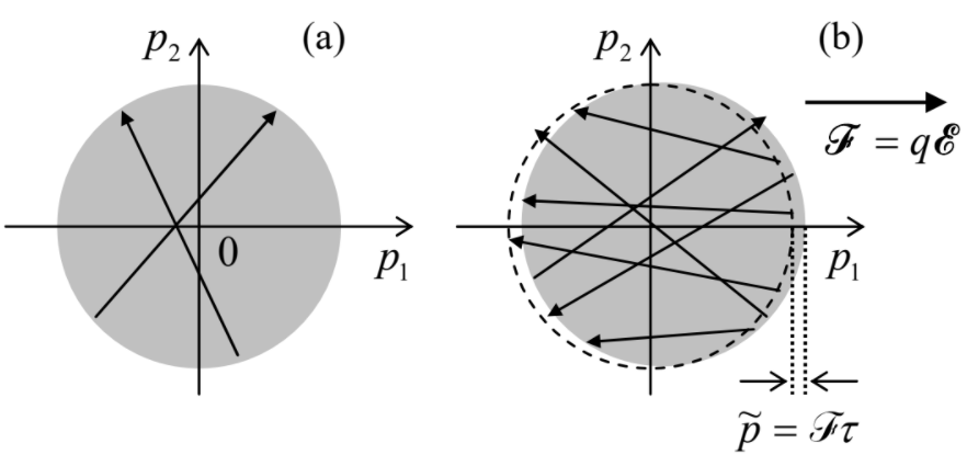
At \(\pmb{\mathscr{E}} = 0\), the system is in equilibrium, so that the quantum states inside the Fermi sphere \((p < p_F)\), are occupied, while those outside of it are empty – see Figure \(\PageIndex{1a}\). Electron scattering events may happen only between states within a very thin layer \((| p^2/2m – \varepsilon_F | \sim T)\) at the Fermi surface, because only in this layer the states are partially occupied, so that both components of the product \(w(\mathbf{r}, \mathbf{p}, t)[1 – w(\mathbf{r}, \mathbf{p}', t)]\), mentioned in Sec. 1, do not vanish. These scattering events, on average, do not change the equilibrium probability distribution, because they are uniformly spread over the Fermi surface.

Now let the electric field be turned on instantly. Immediately it starts accelerating all electrons in its direction, i.e. the whole Fermi sphere starts moving in the momentum space, along the field's direction in the real space. For elastic scattering events (with \(| \mathbf{p}' | = | \mathbf{p} |\)), this creates an addition of occupied states at the leading edge of the accelerating sphere and an addition of free states on its trailing edge (Figure \(\PageIndex{1b}\)). As a result, now there are more scattering events bringing electrons from the leading edge to the trailing edge of the sphere than in the opposite direction. This creates the average backflow of the state occupancy in the momentum space. These two trends eventually cancel each other, and the Fermi sphere approaches a stationary (though not a thermal-equilibrium!) state, with the shift (\ref{35}) relatively to its thermal-equilibrium position.

Now Figure \(\PageIndex{1b}\) may be used to answer the question of which of the two different interpretations of the Drude formula is correct, and the answer is: either. On one hand, we can look at the electric current as a result of the shift (\ref{35}) of all electrons in the momentum space. On the other hand, each filled quantum state deep inside the sphere gives exactly the same contribution to the net current density as it did without the field. All these internal contributions to the net current cancel each other so that the applied field changes the situation only at the Fermi surface. Thus it is equally legitimate to say that only the surface states are responsible for the non-zero net current.¹⁹

Let me also mention another paradox related to the Drude formula, which is often misunderstood (not only by students :-). As was emphasized above, \(\tau\) is finite even at elastic scattering – that by itself does not change the total energy of the gas. The question is how can such scattering be responsible for the Ohmic resistivity \(\rho \equiv 1/\sigma \), and hence for the Joule heat production, with the power density \(\mathscr{p} = \mathbf{j}\cdot \pmb{\mathscr{E}} = \rho j^2\)?²⁰ The answer is that the Drude/Sommerfeld formulas describe just the “bottleneck” of the Joule heat formation. In the scattering picture (Figure \(\PageIndex{1b}\)) the states filled by elastically scattered electrons are located above the (shifted) Fermi surface, and these electrons eventually need to relax onto it via some inelastic process, which releases their excessive energy in the form of heat (in solid state, described by phonons – see Sec. 2.6). The rate and other features of these inelastic phenomena do not participate in the Drude formula directly, but for keeping the theory valid (in particular, keeping the probability distribution w close to its equilibrium value \(w_0\)), their intensity has to be sufficient to avoid gas overheating by the applied field. In some poorly conducting materials, charge carrier overheating effects, resulting in deviations from the Ohm law, i.e. from the linear relation (\ref{28}) between \(\mathbf{j}\) and \(\pmb{\mathscr{E}}\), may be observed already at rather practicable electric fields.

One final comment is that the Sommerfeld theory of the Ohmic conductivity works very well for the electron gas in most conductors. The scheme shown in Figure \(\PageIndex{1}\) helps to understand why: for degenerate Fermi gases the energies of all particles whose scattering contributes to transport properties, are close \((\varepsilon \approx \varepsilon_F)\) and prescribing them all the same relaxation time \(\tau\) is very reasonable. In contrast, in classical gases, with their relatively broad distribution of \(\varepsilon \), some results given by the Boltzmann-RTA equation (\(6.1.18\)) are valid only by the order of magnitude.