6.3: Electrochemical potential and drift-diffusion equation

Now let us generalize our calculation to the case when the particle transport takes place in the presence of a time-independent spatial gradient of the probability distribution, \(\nabla_rw \neq 0\), caused for example by that of the particle concentration \(n = N/V\) (and hence, according to Equation (\(3.2.11\)), of the chemical potential \(\mu \)), while still assuming that temperature \(T\) is constant. For this generalization, we should keep the second term on the left-hand side of Equation (\(6.1.18\)). If the gradient of \(w\) is sufficiently small, we can repeat the arguments of the last section and replace \(w\) with \(w_0\) in this term as well. With the applied electric field \(\pmb{\mathscr{E}}\) represented as \((–\nabla \phi )\),²¹ where \(\phi\) is the electrostatic potential, Equation (\(6.2.7\)) becomes

\[\tilde{w} = \tau \mathbf{v} \cdot \left( \frac{\partial w_0}{\partial \varepsilon} q \nabla \phi - \nabla w_0 \right). \label{36}\]

Since in any of the equilibrium distributions (\(6.2.2\)), \(\langle N(\varepsilon )\rangle\) is a function of \(\varepsilon\) and \(\mu\) only in the combination \((\varepsilon – \mu )\), it obeys the following relation:

\[\frac{\partial \langle N (\varepsilon ) \rangle}{\partial \mu } = - \frac{\partial \langle N (\varepsilon ) \rangle }{\partial \varepsilon}.\label{37}\]

\[\nabla w_0 = - \frac{\partial w_0}{\partial \varepsilon } \nabla \mu, \quad \text{ for } T = \text{ const}, \label{38}\]

so that Equation (\ref{36}) becomes

\[\tilde{w} = \tau \frac{\partial w_0}{\partial \varepsilon} \mathbf{V} \cdot ( q \nabla \phi + \nabla \mu ) \equiv \tau \frac{\partial w_0}{\partial \varepsilon} \mathbf{v} \cdot \nabla \mu ' , \label{39}\]

where the following sum,

Electrochemical potential:

\[\boxed{\mu ' \equiv \mu + q \phi , } \label{40}\]

is called the electrochemical potential. Now repeating the calculation of the electric current, carried out in the last section, we get the following generalization of the Ohm law (\(6.2.10\)):

\[\mathbf{j} = \sigma (− \nabla \mu ' / q) \equiv \sigma \mathcal{E} , \label{41}\]

where the effective electric field \(\mathcal{E}\) is proportional to the gradient of the electrochemical potential, rather of the electrostatic potential:

Effective electric field:

\[\boxed{ \mathcal{E} \equiv - \frac{\nabla \mu '}{q} = \pmb{\mathscr{E}} - \frac{\nabla \mu}{q} .} \label{42}\]

The physics of this extremely important and general result²³ may be explained in two ways. First, let us have a look at the energy spectrum of a degenerate Fermi-gas confined in a volume of finite size, but otherwise free. To ensure such a confinement we need a piecewise-constant potential \(U(\mathbf{r})\) – a “hard-wall, flat-bottom potential well” – see Figure \(\PageIndex{1a}\). (For conduction electrons in a metal, such profile is provided by the positively charged ions of the crystal lattice.) The well should be of a sufficient depth \(U_0 > \varepsilon_F \equiv \mu |_{T = 0}\) to provide the confinement of the overwhelming majority of the particles, with energies below and somewhat above the Fermi level \(\varepsilon_F\). This means that there should be a substantial energy gap,

\[ \Psi \equiv U_0 − \mu >> T , \label{43}\]

between the Fermi energy of a particle inside the well, and its potential energy \(U_0\) outside the well. (The latter value of energy is usually called the vacuum level.) The difference defined by Equation (\ref{43}) is called the workfunction;²⁴ for most metals, it is between 4 and 5 eV, so that the relation \(\Psi >> T\) is well fulfilled for room temperatures (\(T \sim 0.025\) eV) – and actually for all temperatures up to the metal's evaporation point.

Figure \(\PageIndex{1}\): Potential profiles of (a) a single conductor and (b, c) a system of two closely located conductors, for two different biasing situations: (b) zero electrostatic field (the “flat-band condition”), and (c) zero voltage \(\Delta \mu '\).

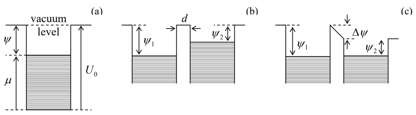
Now let us consider two conductors, with different values of \(\Psi \), separated by a small spatial gap \(d\) – see Figs. \(\PageIndex{1b,c}\). Panel (b) shows the case when the electric field \(\pmb{\mathscr{E}} = –\nabla \phi\) in the free-space gap between the conductors equals zero, i.e. their electrostatic potentials \(\phi\) are equal.²⁵ If there is an opportunity for particles to cross the gap (e.g., by either the thermally-activated hopping over the potential barrier, discussed in Secs. 5.6-5.7, or the quantum-mechanical tunneling through it), there will be an average flow of particles from the conductor with the higher Fermi level to that with the lower Fermi level,²⁶ because the chemical equilibrium requires their equality – see Secs. 1.5 and 2.7. If the particles have an electric charge (as electrons do), the equilibrium will be automatically achieved by them recharging the effective capacitor formed by the conductors, until the electrostatic energy difference \(q\Delta \phi\) reaches the value reproducing that of the workfunctions (Figure \(\PageIndex{1c}\)). So for the equilibrium potential difference²⁷ we may write

\[ q\Delta \phi = \Delta \Psi = −\Delta \mu . \label{44}\]

At this equilibrium, the electric field in the gap between the conductors is

\[\pmb{\mathscr{E}} = -\frac{\Delta \phi}{d}\mathbf{n} = \frac{\Delta \mu}{qd} \mathbf{n} = \frac{\nabla \mu}{q} ; \label{45}\]

in Figure \(\PageIndex{1c}\) this field is clearly visible as the tilt of the electric potential profile. Comparing Equation (\ref{45}) with the definition (\ref{42}) of the effective electric field \(\mathcal{E}\), we see that the equilibrium, i.e. the absence of current through the potential barrier, is achieved exactly when \(\mathcal{E} = 0\), in accordance with Equation (\ref{41}).

The electric field dichotomy, \(\pmb{\mathscr{E}} \leftrightarrow \mathcal{E}\), raises a natural question: which of these fields we are speaking about in the everyday and laboratory practice? Upon some contemplation, the reader should agree that most of our electric field measurements are done indirectly, by measuring corresponding voltages – with voltmeters. A vast majority of these instruments belong to the so-called electrodynamic variety, which is based on the measurement of a small current flowing through the voltmeter.²⁸ As Equation (\ref{41}) shows, such electrodynamic voltmeters measure the electrochemical potential difference \(\Delta \mu '/q\). However, there exists a rare breed of electrostatic voltmeters (also called “electrometers”) that measure the electrostatic potential difference \(\Delta \phi\) between two conductors. One way to implement such an instrument is to use an ordinary, electrodynamic voltmeter, but with the reference point set at the flat band condition (Figure \(\PageIndex{1b}\)) between the conductors. (This condition may be detected by vanishing electric charge on the adjacent surfaces of the conductors, and hence by the absence of its modulation in time if the distance between the surfaces is periodically modulated.)

Now let me return to Equation (\ref{41}) and make two very important remarks. First, it says that in the presence of an electric field, the current vanishes only if \(\nabla \mu ' = 0\), i.e. that the electrochemical potential \(\mu '\), rather than the chemical potential \(\mu \), has to be position-independent in a system in thermodynamic (thermal, chemical, and electric) equilibrium of a conducting system. This result by no means contradicts the fundamental thermodynamic relations for \(\mu\) discussed in Sec. 1.5, or the statistical relations involving \(\mu \), which were discussed in Sec. 2.7 and beyond. Indeed, according to Equation (\ref{40}), \(\mu '(\mathbf{r})\) is “merely” the chemical potential referred to the local value of the electrostatic energy \(q\phi (\mathbf{r})\), and in all previous parts of the course, this energy was assumed to be constant through the system.

Second, note another interpretation of Equation (\ref{41}), which may be achieved by modifying Equation (\ref{38}) for the particular case of the classical gas. Indeed, the local density \(n \equiv N/V\) of the gas obeys Equation (\(3.2.1-3.2.2\)), which may be rewritten as

\[n(\mathbf{r}) = \text{const}\times\exp \left\{\frac{\mu (\mathbf{r})}{T}\right\}. \label{46}\]

Taking the spatial gradient of both sides of this relation (still at constant \(T\)), we get

\[\nabla n = \text{const}\times \frac{1}{T} \exp \left\{\frac{\mu}{T}\right\} \nabla \mu = \frac{n}{T} \nabla \mu , \label{47}\]

so that \(\nabla \mu = (T/n)\nabla n\), and Equation (\ref{41}), with \(\sigma\) given by Equation (\(6.2.14\)), may be recast as

\[\mathbf{j} = \sigma \left(-\frac{\nabla \mu '}{q}\right) \equiv \frac{q^2 \tau}{m} n \left( - \nabla \phi - \frac{1}{q} \nabla \mu \right) \equiv q \frac{\tau}{m} ( nq \pmb{\mathscr{E}} - T \nabla n ). \label{48}\]

Hence the current density may be viewed as consisting of two independent parts: one due to particle drift induced by the “usual” electric field \(\pmb{\mathscr{E}} = –\nabla \phi \), and another due to their diffusion – see Equation (\(5.6.14\)) and its discussion. This is exactly the physics of the “mysterious” term \(\nabla \mu\) in Equation (\ref{42}), though its simple form (\ref{48}) is valid only in the classical limit.

\[\frac{\partial (qn)}{\partial t} + \nabla \cdot \mathbf{j} = 0, \label{49}\]

we get (after the division of all terms by \(q\tau /m\)) the so-called drift-diffusion equation:³⁰

Drift-diffusion equation:

\[\boxed{ \frac{m}{\tau} \frac{\partial n}{\partial t} = \nabla (n \nabla U ) + T \nabla^2 n, \quad \text{ with } U \equiv q \phi . } \label{50}\]

Comparing it with Equation (\(5.6.18\)), we see that the drift-diffusion equation is identical to the Smoluchowski equation,³¹ provided that we parallel the ratio \(\tau /m\) with the mobility \(\mu_m = 1/\eta\) of the Brownian particle. Now using the Einstein relation (\(5.5.17\)), we see that the effective diffusion constant \(D\) of the classical gas of similar particles is

\[D = \frac{\tau T}{m}. \label{51a}\]

This important relation is more frequently represented in either of two other forms. First, since the rare scattering events we are considering do not change the statistics of the gas in thermal equilibrium, we may still use the Maxwell-distribution result (\(3.1.9\)) for the average-square velocity \(\langle v^2\rangle \), to recast Equation (\ref{51a}) as

\[D=\frac{1}{3} \langle v^2 \rangle \tau . \label{51b}\]

One more popular form of the same relation uses the notion of the mean free path \(l\), which may be defined as the average distance passed by the particle between two sequential scattering events:

\[D=\frac{1}{3} l \langle v^2 \rangle^{1/2} , \quad \text{ with } l \equiv \langle v^2 \rangle^{1/2} \tau . \label{51c}\]

In the forms (\ref{51b})-(\ref{51c}), the result for \(D\) makes more physical sense, because it may be readily derived (admittedly, with some uncertainty of the numerical coefficient) from simple kinematic arguments – the task left for the reader's exercise. Note that since the definition of \(\tau\) in Equation (\(6.1.17\)) is phenomenological, so is the above definition of \(l\); this is why several definitions of this parameter, which may differ by a numerical factor of the order of 1, are possible.

Note also that using Equation (\ref{51a}), Equation (\ref{48}) may be rewritten as an expression for the particle flow density \(\mathbf{j}_n \equiv n \mathbf{j}_w = \mathbf{j} / q\):

\[ \mathbf{j}_n = n \mu_m q \pmb{\mathscr{E}} - D \nabla n, \label{52}\]

with the first term on the right-hand side describing particles' drift, while the second one, their diffusion. I will discuss the application of this equation to the most important case of non-degenerate (“quasi classical”) gases of electrons and holes in semiconductors, in the next section.

To complete this section, let me emphasize again that the mathematically similar drift-diffusion equation (\ref{50}) and the Smoluchowski equation (\(5.6.18\)) describe different physical situations. Indeed, our (or rather Einstein and Smoluchowski's :-) treatment of the Brownian motion in Chapter 5 was based on a strong hierarchy of the system, consisting of a large “Brownian particle” in an environment of many smaller particles – “molecules”. On the other hand, in this chapter we are considering a gas of similar particles. Nevertheless, the equations describing the dynamics of their probability distribution, are the same – at least within the framework of the Boltzmann transport equation with the relaxation-time approximation (\(6.1.17\)) of the scattering integral. The origin of this similarity is the fact that Equation (\(6.1.12\)) is clearly applicable to a Brownian particle as well, with each “scattering” event being the particle's hit by a random molecule of its environment. Since, due to the mass hierarchy, the particle momentum change at each such event is very small, the scattering integral has to be local, i.e. depend only on w at the same momentum \(\mathbf{p}\) as the left-hand side of the Boltzmann equation, so that the relaxation time approximation (\(6.1.17\)) is absolutely natural – indeed, more natural than for our current case of similar particles.