
6.1: The Liouville Theorem and the Boltzmann Rquation


- Last updated
- Sep 20, 2022
- Save as PDF

( \newcommand{\kernel}{\mathrm{null}\,}\)
Physical kinetics (not to be confused with “kinematics”!) is the branch of statistical physics that deals with systems out of thermodynamic equilibrium. Major effects addressed by kinetics include:
- for autonomous systems (those out of external fields): the transient processes (relaxation), that lead from an arbitrary initial state of a system to its thermodynamic equilibrium;
- for systems in time-dependent (say, sinusoidal) external fields: the field-induced periodic oscillations of the system's variables; and
- for systems in time-independent (“dc”) external fields: dc transport.
In the last case, we are dealing with stationary (∂/∂t=0 everywhere), but non-equilibrium situations, in which the effect of an external field, continuously driving the system out of equilibrium, is balanced by the simultaneous relaxation – the trend back to equilibrium. Perhaps the most important effect of this class is the dc current in conductors and semiconductors,1 which alone justifies the inclusion of the basic notions of kinetics into any set of core physics courses.
The reader who has reached this point of the notes already has some taste of physical kinetics, because the subject of the last part of Chapter 5 was the kinetics of a “Brownian particle”, i.e. of a “heavy” system interacting with an environment consisting of many “lighter” components. Indeed, the equations discussed in that part – whether the Smoluchowski equation (5.6.18) or the Fokker-Planck equation (5.7.11) – are valid if the environment is in thermodynamic equilibrium, but the system of our interest is not necessarily so. As a result, we could use those equations to discuss such non-equilibrium phenomena as the Kramers problem of the metastable state's lifetime.
In contrast, this chapter is devoted to the more traditional subject of kinetics: systems of many similar particles – generally, interacting with each other, but not too strongly, so that the energy of the system still may be partitioned into a sum of single-particle components, with the interparticle interactions considered as a weak perturbation. Actually, we have already started the job of describing such a system at the beginning of Sec. 5.7. Indeed, in the absence of particle interactions (i.e. when it is unimportant whether the particle of our interest is “light” or “heavy”), the probability current densities in the coordinate and momentum spaces are given, respectively, by Equation (5.7.3) and the first form of Equation (5.7.4), so that the continuity equation (5.7.1) takes the form
∂w∂t+∇q⋅(w˙q)+∇p⋅(w˙p)=0.
If similar particles do not interact, this equation for the single-particle probability density w(q,p,t) is valid for each of them, and the result of its solution may be used to calculate any ensemble-average characteristic of the system as a whole.
Let us rewrite Equation (???) in the Cartesian-component form,
∂w∂t+∑j[∂∂qj(w˙qj)+∂∂pj(w˙pj)]=0,
˙qj=∂H∂pj,˙pj=−∂H∂qj,
We get
∂w∂t+∑j[∂∂qj(w∂H∂pj)−∂∂pj(w∂H∂qj)]=0.
Liouville theorem:
∂w∂t+∑j(∂w∂qj˙qj+∂w∂pj˙pj)=0.
Since the left-hand side of this equation is just the full derivative of the probability density w considered as a function of the generalized coordinates qj(t) of a particle, its generalized momenta components pj(t), and (possibly) time t,4 the Liouville theorem (???) may be represented in a surprisingly simple form:
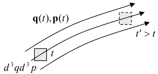
dw(q,p,t)dt=0.
Physically this means that the elementary probability dW=wd3qd3p to find a Hamiltonian particle in a small volume of the coordinate-momentum space [q,p], with its center moving in accordance to the deterministic law (???), does not change with time – see Figure 6.1.1.
At the first glance, this may not look surprising because according to the fundamental Einstein relation (5.5.17), one needs non-Hamiltonian forces (such as the kinematic friction) to have diffusion. On the other hand, it is striking that the Liouville theorem is valid even for (Hamiltonian) systems with deterministic chaos,5 in which the deterministic trajectories corresponding to slightly different initial conditions become increasingly mixed with time.
For an ideal gas of 3D particles, we may use the ordinary Cartesian coordinates rj (with j=1,2,3) for the generalized coordinates qj, so that pj become the Cartesian components mvj of the usual (linear) momentum, and the elementary volume is just d3rd3p – see Figure 6.1.1. In this case, Eqs. (???) are just
˙rj=pjm≡vj,˙pj=Fj,
where FF is the force exerted on the particle, so that the Liouville theorem may be rewritten as
∂w∂t+3∑j=1(vj∂w∂rj+Fj∂w∂pj)=0,
and conveniently represented in the vector form
∂w∂t+v⋅∇rw+FF⋅∇pw=0.
Of course, the situation becomes much more complex if the particles interact. Generally, a system of N similar particles in 3D space has to be described by the probability density being a function of 6N+1 arguments (3N Cartesian coordinates, plus 3N momentum components, plus time). An analytical or numerical solution of any equation describing the time evolution of such a function for a typical system of N∼1023 particles is evidently a hopeless task. Hence, any theory of realistic systems' kinetics has to rely on making reasonable approximations that would simplify the situation.
One of the most useful approximations (sometimes called Stosszahlansatz – German for the “collision-number assumption”) was suggested by Ludwig Boltzmann for gas of particles that move freely most of the time but interact during short time intervals, when a particle comes close to either an immobile scattering center (say, an impurity in a conductor's crystal lattice) or to another particle of the gas. Such brief scattering events may change the particle's momentum. Boltzmann argued that they may be still approximately described Equation (???), with the addition of a special term (called the scattering integral) to its right-hand side:
Boltzmann equation:
∂w∂t+v⋅∇rw+FF⋅∇pw=∂w∂t|scattering.
This is the Boltzmann equation, also called the “Boltzmann transport equation”. As will be discussed below, it may give a very reasonable description of not only classical but also quantum particles, though it evidently neglects the quantum-mechanical coherence/entanglement effects6 – besides those that may be hidden inside the scattering integral.
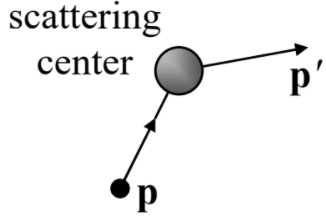
The concrete form of the scattering integral depends on the type of particle scattering. If the scattering centers do not belong to the ensemble under consideration (an example is given, again, by impurity atoms in a conductor), then the scattering integral may be expressed as an evident generalization of the master equation (4.5.24):
∂w∂t|scattering=∫d3p′[Γp′→pw(r,p′,t)−Γp→p′w(r,p,t)],
where the physical sense of Γp→p′ is the rate (i.e. the probability per unit time) for the particle to be scattered from the state with the momentum p into the state with the momentum p′ – see Figure 6.1.2.
Most elastic interactions are reciprocal, i.e. obey the following relation (closely related to the reversibility of time in Hamiltonian systems): Γp→p′=Γp′→p, so that Equation (???) may be rewritten as7
∂w∂t|scattering=∫d3p′Γp→p′[w(r,p′,t)−w(r,p,t)].
With such scattering integral, Equation (???) stays linear in w but becomes an integro-differential equation, typically harder to solve analytically than differential equations.
The equation becomes even more complex if the scattering is due to the mutual interaction of the particle members of the system – see Figure 6.1.3.
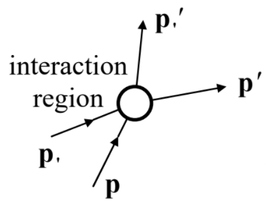
In this case, the probability of a scattering event scales as a product of two single-particle probabilities, and the simplest reasonable form of the scattering integral is8
∂w∂t|scattering=∫d3p′∫d3p⋅[Γp′→p,p′→p,w(r,p′,t)w(r,p′′,t)−Γ′p→p′,p′→p′w(r,p,t)w(r,p′,t)].
The integration dimensionality in Equation (???) takes into account the fact that due to the conservation of the total momentum at scattering,
p+p′=p′+p′′,
one of the momenta is not an independent argument, so that the integration in Equation (???) may be restricted to a 6D p-space rather than the 9D one. For the reciprocal interaction, Equation (???) may also be a bit simplified, but it still keeps Equation (???) a nonlinear integro-differential transport equation, excluding such powerful solution methods as the Fourier expansion – which hinges on the linear superposition principle.
This is why most useful results based on the Boltzmann transport equation depend on its further simplifications, most notably the relaxation-time approximation – RTA for short.9 This approximation is based on the fact that in the absence of spatial gradients (∇=0), and external forces (FF=0), in at the thermal equilibrium, Equation (???) yields
∂w∂t=∂w∂t|scattering,
so that the equilibrium probability distribution w0(r,p,t) has to turn any scattering integral to zero. Hence at a small deviation from the equilibrium,
˜w(r,p,t)≡w(r,p,t)−w0(r,p,t)→0,
the scattering integral should be proportional to the deviation ˜w, and its simplest reasonable model is
Relaxation-time approximation (RTA):
∂w∂t|scattering=−˜wτ,
where τ is a phenomenological constant (which, according to Equation (???), has to be positive for the system's stability) called the relaxation time. Its physical meaning will be more clear in the next section.
The relaxation-time approximation is quite reasonable if the angular distribution of the scattering rate is dominated by small angles between vectors p and p′ – as it is, for example, for the Rutherford scattering by a Coulomb center.10 Indeed, in this case the two values of the function w, participating in Equation (???), are close to each other for most scattering events so that the loss of the second momentum argument (p′) is not too essential. However, using the Boltzmann-RTA equation that results from combining Eqs. (???) and (???),
Boltzmann-RTA equation:
∂w∂t+v⋅∇rw+FF⋅∇pw=−˜wτ,
we should always remember that this is just a phenomenological model, sometimes giving completely wrong results. For example, it prescribes the same time scale (τ) to the relaxation of the net momentum of the system, and to its energy relaxation, while in many real systems the latter process (that results from inelastic collisions) may be substantially longer. Naturally, in the following sections, I will describe only those applications of the Boltzmann-RTA equation that give a reasonable description of physical reality.