Physics LibreTexts

5.10: Sample problems and solutions

  • Page ID
    19396

    \( \newcommand{\vecs}[1]{\overset { \scriptstyle \rightharpoonup} {\mathbf{#1}} } \)

    \( \newcommand{\vecd}[1]{\overset{-\!-\!\rightharpoonup}{\vphantom{a}\smash {#1}}} \)

    \( \newcommand{\id}{\mathrm{id}}\) \( \newcommand{\Span}{\mathrm{span}}\)

    ( \newcommand{\kernel}{\mathrm{null}\,}\) \( \newcommand{\range}{\mathrm{range}\,}\)
    \( \newcommand{\RealPart}{\mathrm{Re}}\) \( \newcommand{\ImaginaryPart}{\mathrm{Im}}\)

    \( \newcommand{\Argument}{\mathrm{Arg}}\) \( \newcommand{\norm}[1]{\| #1 \|}\)

    \( \newcommand{\inner}[2]{\langle #1, #2 \rangle}\)

    \( \newcommand{\Span}{\mathrm{span}}\)

    \( \newcommand{\id}{\mathrm{id}}\)

    \( \newcommand{\Span}{\mathrm{span}}\)

    \( \newcommand{\kernel}{\mathrm{null}\,}\)

    \( \newcommand{\range}{\mathrm{range}\,}\)

    \( \newcommand{\RealPart}{\mathrm{Re}}\)

    \( \newcommand{\ImaginaryPart}{\mathrm{Im}}\)

    \( \newcommand{\Argument}{\mathrm{Arg}}\)

    \( \newcommand{\norm}[1]{\| #1 \|}\)

    \( \newcommand{\inner}[2]{\langle #1, #2 \rangle}\)

    \( \newcommand{\Span}{\mathrm{span}}\) \( \newcommand{\AA}{\unicode[.8,0]{x212B}}\)

    \( \newcommand{\vectorA}[1]{\vec{#1}}      % arrow\)

    \( \newcommand{\vectorAt}[1]{\vec{\text{#1}}}      % arrow\)

    \( \newcommand{\vectorB}[1]{\overset { \scriptstyle \rightharpoonup} {\mathbf{#1}} } \)

    \( \newcommand{\vectorC}[1]{\textbf{#1}} \)

    \( \newcommand{\vectorD}[1]{\overrightarrow{#1}} \)

    \( \newcommand{\vectorDt}[1]{\overrightarrow{\text{#1}}} \)

    \( \newcommand{\vectE}[1]{\overset{-\!-\!\rightharpoonup}{\vphantom{a}\smash{\mathbf {#1}}}} \)

    \( \newcommand{\vecs}[1]{\overset { \scriptstyle \rightharpoonup} {\mathbf{#1}} } \)

    \( \newcommand{\vecd}[1]{\overset{-\!-\!\rightharpoonup}{\vphantom{a}\smash {#1}}} \)

    \(\newcommand{\avec}{\mathbf a}\) \(\newcommand{\bvec}{\mathbf b}\) \(\newcommand{\cvec}{\mathbf c}\) \(\newcommand{\dvec}{\mathbf d}\) \(\newcommand{\dtil}{\widetilde{\mathbf d}}\) \(\newcommand{\evec}{\mathbf e}\) \(\newcommand{\fvec}{\mathbf f}\) \(\newcommand{\nvec}{\mathbf n}\) \(\newcommand{\pvec}{\mathbf p}\) \(\newcommand{\qvec}{\mathbf q}\) \(\newcommand{\svec}{\mathbf s}\) \(\newcommand{\tvec}{\mathbf t}\) \(\newcommand{\uvec}{\mathbf u}\) \(\newcommand{\vvec}{\mathbf v}\) \(\newcommand{\wvec}{\mathbf w}\) \(\newcommand{\xvec}{\mathbf x}\) \(\newcommand{\yvec}{\mathbf y}\) \(\newcommand{\zvec}{\mathbf z}\) \(\newcommand{\rvec}{\mathbf r}\) \(\newcommand{\mvec}{\mathbf m}\) \(\newcommand{\zerovec}{\mathbf 0}\) \(\newcommand{\onevec}{\mathbf 1}\) \(\newcommand{\real}{\mathbb R}\) \(\newcommand{\twovec}[2]{\left[\begin{array}{r}#1 \\ #2 \end{array}\right]}\) \(\newcommand{\ctwovec}[2]{\left[\begin{array}{c}#1 \\ #2 \end{array}\right]}\) \(\newcommand{\threevec}[3]{\left[\begin{array}{r}#1 \\ #2 \\ #3 \end{array}\right]}\) \(\newcommand{\cthreevec}[3]{\left[\begin{array}{c}#1 \\ #2 \\ #3 \end{array}\right]}\) \(\newcommand{\fourvec}[4]{\left[\begin{array}{r}#1 \\ #2 \\ #3 \\ #4 \end{array}\right]}\) \(\newcommand{\cfourvec}[4]{\left[\begin{array}{c}#1 \\ #2 \\ #3 \\ #4 \end{array}\right]}\) \(\newcommand{\fivevec}[5]{\left[\begin{array}{r}#1 \\ #2 \\ #3 \\ #4 \\ #5 \\ \end{array}\right]}\) \(\newcommand{\cfivevec}[5]{\left[\begin{array}{c}#1 \\ #2 \\ #3 \\ #4 \\ #5 \\ \end{array}\right]}\) \(\newcommand{\mattwo}[4]{\left[\begin{array}{rr}#1 \amp #2 \\ #3 \amp #4 \\ \end{array}\right]}\) \(\newcommand{\laspan}[1]{\text{Span}\{#1\}}\) \(\newcommand{\bcal}{\cal B}\) \(\newcommand{\ccal}{\cal C}\) \(\newcommand{\scal}{\cal S}\) \(\newcommand{\wcal}{\cal W}\) \(\newcommand{\ecal}{\cal E}\) \(\newcommand{\coords}[2]{\left\{#1\right\}_{#2}}\) \(\newcommand{\gray}[1]{\color{gray}{#1}}\) \(\newcommand{\lgray}[1]{\color{lightgray}{#1}}\) \(\newcommand{\rank}{\operatorname{rank}}\) \(\newcommand{\row}{\text{Row}}\) \(\newcommand{\col}{\text{Col}}\) \(\renewcommand{\row}{\text{Row}}\) \(\newcommand{\nul}{\text{Nul}}\) \(\newcommand{\var}{\text{Var}}\) \(\newcommand{\corr}{\text{corr}}\) \(\newcommand{\len}[1]{\left|#1\right|}\) \(\newcommand{\bbar}{\overline{\bvec}}\) \(\newcommand{\bhat}{\widehat{\bvec}}\) \(\newcommand{\bperp}{\bvec^\perp}\) \(\newcommand{\xhat}{\widehat{\xvec}}\) \(\newcommand{\vhat}{\widehat{\vvec}}\) \(\newcommand{\uhat}{\widehat{\uvec}}\) \(\newcommand{\what}{\widehat{\wvec}}\) \(\newcommand{\Sighat}{\widehat{\Sigma}}\) \(\newcommand{\lt}{<}\) \(\newcommand{\gt}{>}\) \(\newcommand{\amp}{&}\) \(\definecolor{fillinmathshade}{gray}{0.9}\)
    Exercise \(\PageIndex{1}\)
    clipboard_e22712a6f51dd8108698094a21addc9b4.png
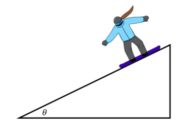
    Figure \(\PageIndex{1}\): Katie snowboarding down an incline.

    Katie, an amateur snowboarder, rests at the top of hill inclined by an angle of \(\theta=50^{\circ}\) with respect to the horizontal, as shown in Figure \(\PageIndex{1}\). She gracefully slides down the hill until she face-plants into a large pile of snow at the bottom, \(40\text{m}\) from where she started. If the coefficient of kinetic friction between Katie’s snowboard and the hill is \(\mu_k=0.45\), how long elapses between when she starts to glide and when she face plants?

    Answer

    Before trying to solve the problem, we should think of the strategy that will allow us to model the time that it takes to arrive at the bottom. We know that Newton’s Second Law relates the forces on Katie to her acceleration. If we build a model of the forces on Katie, we can then determine her acceleration. Once we know her acceleration, we can use kinematics to determine how long it takes for her to cover the distance of \(40\text{m}\).

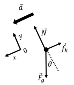
    The forces exerted on Katie are:

    1. \(\vec F_g\), her weight.
    2. \(\vec N\), a normal force exerted by the slope.
    3. \(\vec f_k\), a force of kinetic friction exerted by the slope, with magnitude \(f_k=\mu_kN\)

    This allows us to build a free-body diagram for the forces on Katie, as shown in Figure 5.9.2. Since Katie will glide down the slope, her acceleration will be parallel to the slope and downwards, which we showed with a thicker arrow on the free-body diagram. Our free-body diagram also shows the coordinate system that we chose, with the \(x\) axis pointing parallel to the acceleration.
    clipboard_ef6705ebf3c00c96e4664968e68f4a8f5.png
    Figure \(\PageIndex{2}\): Forces acting on Katie as she snowboards.

    With a free-body diagram, we can write the \(x\) and \(y\) components of Newton’s Second Law. In the \(x\) direction, both the force of friction and the weight have components. The force of friction is in the negative \(x\) direction, whereas the component of gravity in the \(x\) direction is \(F_g\sin\theta\). The acceleration vector is also in the \(x\) direction. Putting this altogether into Newton’s Second Law:

    \[\begin{aligned} \sum F_x = F_g\sin\theta - f_k &= ma\\[4pt] \therefore mg\sin\theta -\mu_k N &= ma\end{aligned}\]

    where we used the fact that the weight is given by \(mg\) (\(m\) is Katie’s mass) and the magnitude of the force of friction is given by \(f_k=\mu_kN\).

    Next, we write out the \(y\) component of Newton’s Second Law. The normal force is in the positive \(y\) direction, whereas the component of gravity in the \(y\) direction is \(-F_g\cos\theta\). The acceleration has no component in the \(y\) direction. Putting this into Newton’s Second Law:

    \[\begin{aligned} \sum F_y = N-F_g\cos\theta &=0\\[4pt] \therefore N-mg\cos\theta &=0\end{aligned}\]

    We now have two equations that describe Katie’s motion:

    \[\begin{aligned} mg\sin\theta -\mu_k N &= ma\\[4pt] N-mg\cos\theta &=0\end{aligned}\]

    We have three unknowns, \(m\), \(N\), and \(a\), but only two equations! Hopefully, one of these will cancel out! At this point, all of the physics for the problem is done! We can now proceed to solve these equations to find the acceleration. The second equation allows us to solve for the normal force, \(N=mg\cos\theta\), which we substitute into the first equation:

    \[\begin{aligned} mg\sin\theta -\mu_k N &= ma\\[4pt] \therefore mg\sin\theta -\mu_k mg\cos\theta &= ma\\[4pt]\end{aligned}\]

    As you can see, the mass \(m\) can be canceled out of this equation, and we can find the acceleration:

    \(\begin{aligned} a&=g\sin\theta-\mu_{k}g\cos\theta \\[4pt] &=g(\sin\theta -\mu_{k}\cos\theta ) \\[4pt] &=(9.8\text{N/kg})(\sin (50^{\circ})-(0.45)\cos (50^{\circ})) \\[4pt] &=4.67\text{N/kg} \end{aligned}\)

    At this point, we should ask ourselves if our result makes sense. In particular, we have found that the acceleration has unit of \(\text{N/kg}\) instead of \(\text{m/s}^{2}\). A quick examination of Newton’s Second Law shows us that these two units are equivalent:

    \[\begin{aligned} F &= ma\\[4pt] a &= \frac{F}{m}\\[4pt] \therefore SI[a] &= \frac{SI[F]}{SI[m]}=\frac{\text{N}}{\text{kg}}\end{aligned}\]

    Often, one write the magnitude of the Earth’s gravitation field as \(g=9.8\text{m/s}^{2}\), since it has the same dimension as acceleration, and does indeed correspond to the acceleration that is felt by falling objects near the surface of the Earth. In fact, \(g\), is usually defined as the acceleration of object near the Earth, although this is misleading, as it requires that inertial and gravitational mass be the same.

    Knowing that Katie’s initial velocity is \(v_{0x}=0\text{m/s}\), her acceleration is \(a_x=a=4.67\text{m/s}^{2}\) in the \(x\) direction (the same direction as the slope), and the distance that she must travel is \(x=40\text{m}\), we can find the time it takes for her to face-plant. If we set the origin of the \(x\) axis where she starts (so that her initial position along the \(x\) axis, \(x_0=0\)), the distance that she covered in the time, \(t\), is given by:

    \[\begin{aligned} x(t)&=x_0+v_{0x}t+\frac{1}{2}at^2\\[4pt] 40\text{m}&=(0)+(0)t+\frac{1}{2}(1.31\text{m/s}^{2})t^2\\[4pt] \therefore t&=\sqrt{\frac{2(40\text{m})}{(4.67\text{m/s}^{2})}}=4.14\text{s}\end{aligned}\]

    Katie has \(4.14\text{s}\) of gliding bliss before face-planting into the large pile of snow.
    Exercise \(\PageIndex{2}\)
    clipboard_ea2b64011188e6fce291d950ca9223a0a.png
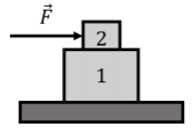
    Figure \(\PageIndex{3}\): Two stacked boxes.

    Two boxes with masses, \(m_1\) and \(m_2\), respectively, are placed on top of one another, as shown in Figure \(\PageIndex{3}\). The coefficient of static friction between the two boxes and between the boxes and the ground is \(\mu_s=0.3\). A constant force, \(\vec F\), is exerted on box 2, as shown. Show that it is impossible for box 1 to accelerate.

    Answer

    The only way for box 1 to accelerate is if box 2 “drags” box 1 along with it through a force of friction exerted at the interface between box 1 and box 2. We need to show that the force of (static) friction exerted by the ground on box 1 will always be at least as large as the force of friction exerted by box 2 on box 1. The largest force of friction that box 2 can exert on box 1 is a force of static friction, so we model all forces between surfaces as forces of static friction.

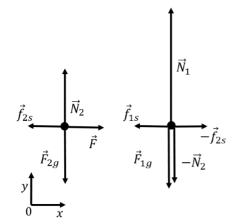
    The forces on box 2 are:

    • \(\vec F_{2g}\), its weight.
    • \(\vec N_2\), a normal exerted by box 1.
    • \(\vec f_{2s}\), a force of static friction exerted by box 1.
    • \(\vec F\), the applied force.

    The forces on box 1 are:

    • \(\vec F_{1g}\), its weight.
    • \(-\vec N_2\), a normal force exerted by box 2 (downwards).
    • \(-\vec f_{2s}\), a force of static friction exerted by box 2.
    • \(\vec N_1\), a normal force exerted by the ground.
    • \(\vec f_{1s}\), a force of static friction exerted by the ground.

    The are illustrated in the free-body diagram in Figure \(\PageIndex{4}\).

    clipboard_e4f492922eb967e1370322fbecffd53bf.png
    Figure \(\PageIndex{4}\): Forces on the two boxes.

    Considering the \(y\) component of Newton’s Second Law for box 2 (the top box), we can find the value of the normal force exerted by box 1:

    \[\begin{aligned} \sum F_y &= N_2 - F_{2g} = 0\\[4pt] \therefore N_2 &= m_2 g\end{aligned}\]

    The maximal magnitude of the force of static friction, \(f_{2s}\), between the two boxes is given by:

    \[\begin{aligned} f_{2s} = \mu_sN_2 = \mu_s m_2g\end{aligned}\]

    This is the maximal magnitude of the force that can accelerate box 1. Considering the \(y\) component of Newton’s Second Law applied to box 1, we can find \(N_1\), the normal force exerted by the ground:

    \[\begin{aligned} \sum F_y = N_1 - F_{1g} - N_2 = 0\\[4pt] \therefore N_1 = F_{1g}+N_2 = (m_1+m_2)g\end{aligned}\]

    The force of static friction exerted by the ground on box 1 will be in the opposite direction as the force of static friction exerted by box 2. The maximal magnitude of the force of static friction exerted by the ground is given by:

    \[\begin{aligned} f_{1s} = \mu_sN_1 = \mu_s (m_1+m_2)g\end{aligned}\]

    We can see that the maximal force of static friction exerted by the ground will always exceed the magnitude of the force of static friction exerted by box 2. It is thus impossible to push on box 2 to make box 1 move (as long as the force of static friction between the two boxes and the box and the ground are the same).


    This page titled 5.10: Sample problems and solutions is shared under a CC BY-SA 4.0 license and was authored, remixed, and/or curated by Ryan D. Martin, Emma Neary, Joshua Rinaldo, and Olivia Woodman via source content that was edited to the style and standards of the LibreTexts platform.