
18.2: Electric potential
- Page ID
- 19496

\( \newcommand{\vecs}[1]{\overset { \scriptstyle \rightharpoonup} {\mathbf{#1}} } \)
\( \newcommand{\vecd}[1]{\overset{-\!-\!\rightharpoonup}{\vphantom{a}\smash {#1}}} \)
\( \newcommand{\dsum}{\displaystyle\sum\limits} \)
\( \newcommand{\dint}{\displaystyle\int\limits} \)
\( \newcommand{\dlim}{\displaystyle\lim\limits} \)
\( \newcommand{\id}{\mathrm{id}}\) \( \newcommand{\Span}{\mathrm{span}}\)
( \newcommand{\kernel}{\mathrm{null}\,}\) \( \newcommand{\range}{\mathrm{range}\,}\)
\( \newcommand{\RealPart}{\mathrm{Re}}\) \( \newcommand{\ImaginaryPart}{\mathrm{Im}}\)
\( \newcommand{\Argument}{\mathrm{Arg}}\) \( \newcommand{\norm}[1]{\| #1 \|}\)
\( \newcommand{\inner}[2]{\langle #1, #2 \rangle}\)
\( \newcommand{\Span}{\mathrm{span}}\)
\( \newcommand{\id}{\mathrm{id}}\)
\( \newcommand{\Span}{\mathrm{span}}\)
\( \newcommand{\kernel}{\mathrm{null}\,}\)
\( \newcommand{\range}{\mathrm{range}\,}\)
\( \newcommand{\RealPart}{\mathrm{Re}}\)
\( \newcommand{\ImaginaryPart}{\mathrm{Im}}\)
\( \newcommand{\Argument}{\mathrm{Arg}}\)
\( \newcommand{\norm}[1]{\| #1 \|}\)
\( \newcommand{\inner}[2]{\langle #1, #2 \rangle}\)
\( \newcommand{\Span}{\mathrm{span}}\) \( \newcommand{\AA}{\unicode[.8,0]{x212B}}\)
\( \newcommand{\vectorA}[1]{\vec{#1}} % arrow\)
\( \newcommand{\vectorAt}[1]{\vec{\text{#1}}} % arrow\)
\( \newcommand{\vectorB}[1]{\overset { \scriptstyle \rightharpoonup} {\mathbf{#1}} } \)
\( \newcommand{\vectorC}[1]{\textbf{#1}} \)
\( \newcommand{\vectorD}[1]{\overrightarrow{#1}} \)
\( \newcommand{\vectorDt}[1]{\overrightarrow{\text{#1}}} \)
\( \newcommand{\vectE}[1]{\overset{-\!-\!\rightharpoonup}{\vphantom{a}\smash{\mathbf {#1}}}} \)
\( \newcommand{\vecs}[1]{\overset { \scriptstyle \rightharpoonup} {\mathbf{#1}} } \)
\(\newcommand{\longvect}{\overrightarrow}\)
\( \newcommand{\vecd}[1]{\overset{-\!-\!\rightharpoonup}{\vphantom{a}\smash {#1}}} \)
\(\newcommand{\avec}{\mathbf a}\) \(\newcommand{\bvec}{\mathbf b}\) \(\newcommand{\cvec}{\mathbf c}\) \(\newcommand{\dvec}{\mathbf d}\) \(\newcommand{\dtil}{\widetilde{\mathbf d}}\) \(\newcommand{\evec}{\mathbf e}\) \(\newcommand{\fvec}{\mathbf f}\) \(\newcommand{\nvec}{\mathbf n}\) \(\newcommand{\pvec}{\mathbf p}\) \(\newcommand{\qvec}{\mathbf q}\) \(\newcommand{\svec}{\mathbf s}\) \(\newcommand{\tvec}{\mathbf t}\) \(\newcommand{\uvec}{\mathbf u}\) \(\newcommand{\vvec}{\mathbf v}\) \(\newcommand{\wvec}{\mathbf w}\) \(\newcommand{\xvec}{\mathbf x}\) \(\newcommand{\yvec}{\mathbf y}\) \(\newcommand{\zvec}{\mathbf z}\) \(\newcommand{\rvec}{\mathbf r}\) \(\newcommand{\mvec}{\mathbf m}\) \(\newcommand{\zerovec}{\mathbf 0}\) \(\newcommand{\onevec}{\mathbf 1}\) \(\newcommand{\real}{\mathbb R}\) \(\newcommand{\twovec}[2]{\left[\begin{array}{r}#1 \\ #2 \end{array}\right]}\) \(\newcommand{\ctwovec}[2]{\left[\begin{array}{c}#1 \\ #2 \end{array}\right]}\) \(\newcommand{\threevec}[3]{\left[\begin{array}{r}#1 \\ #2 \\ #3 \end{array}\right]}\) \(\newcommand{\cthreevec}[3]{\left[\begin{array}{c}#1 \\ #2 \\ #3 \end{array}\right]}\) \(\newcommand{\fourvec}[4]{\left[\begin{array}{r}#1 \\ #2 \\ #3 \\ #4 \end{array}\right]}\) \(\newcommand{\cfourvec}[4]{\left[\begin{array}{c}#1 \\ #2 \\ #3 \\ #4 \end{array}\right]}\) \(\newcommand{\fivevec}[5]{\left[\begin{array}{r}#1 \\ #2 \\ #3 \\ #4 \\ #5 \\ \end{array}\right]}\) \(\newcommand{\cfivevec}[5]{\left[\begin{array}{c}#1 \\ #2 \\ #3 \\ #4 \\ #5 \\ \end{array}\right]}\) \(\newcommand{\mattwo}[4]{\left[\begin{array}{rr}#1 \amp #2 \\ #3 \amp #4 \\ \end{array}\right]}\) \(\newcommand{\laspan}[1]{\text{Span}\{#1\}}\) \(\newcommand{\bcal}{\cal B}\) \(\newcommand{\ccal}{\cal C}\) \(\newcommand{\scal}{\cal S}\) \(\newcommand{\wcal}{\cal W}\) \(\newcommand{\ecal}{\cal E}\) \(\newcommand{\coords}[2]{\left\{#1\right\}_{#2}}\) \(\newcommand{\gray}[1]{\color{gray}{#1}}\) \(\newcommand{\lgray}[1]{\color{lightgray}{#1}}\) \(\newcommand{\rank}{\operatorname{rank}}\) \(\newcommand{\row}{\text{Row}}\) \(\newcommand{\col}{\text{Col}}\) \(\renewcommand{\row}{\text{Row}}\) \(\newcommand{\nul}{\text{Nul}}\) \(\newcommand{\var}{\text{Var}}\) \(\newcommand{\corr}{\text{corr}}\) \(\newcommand{\len}[1]{\left|#1\right|}\) \(\newcommand{\bbar}{\overline{\bvec}}\) \(\newcommand{\bhat}{\widehat{\bvec}}\) \(\newcommand{\bperp}{\bvec^\perp}\) \(\newcommand{\xhat}{\widehat{\xvec}}\) \(\newcommand{\vhat}{\widehat{\vvec}}\) \(\newcommand{\uhat}{\widehat{\uvec}}\) \(\newcommand{\what}{\widehat{\wvec}}\) \(\newcommand{\Sighat}{\widehat{\Sigma}}\) \(\newcommand{\lt}{<}\) \(\newcommand{\gt}{>}\) \(\newcommand{\amp}{&}\) \(\definecolor{fillinmathshade}{gray}{0.9}\)As you recall, we defined the electric field, \(\vec E(\vec r)\), to be the electric force per unit charge. By defining an electric field everywhere in space, we were able to easily determine the force on any test charge, \(q\), whether the test charge is positive or negative (since the sign of \(q\) will change the direction of the force vector, \(q\vec E\)):
\[\begin{aligned} \vec E(\vec r) &= \frac{\vec F^E(\vec r)}{q}\\[4pt] \therefore \vec F^E(\vec r)&=q\vec E(\vec r)\end{aligned}\]
Similarly, we define the electric potential, \(V(\vec r)\), to be the electric potential energy per unit charge. This allows us to define electric potential, \(V(\vec r)\), everywhere in space, and then determine the potential energy of a specific charge, \(q\), by simply multiplying \(q\) with the electric potential at that position in space.
\[\begin{aligned} V(\vec r) &= \frac{ U(\vec r)}{q}\\[4pt] \therefore U(\vec r)&= q V(\vec r)\end{aligned}\]
The S.I. unit for electric potential is the “volt”, (V). Electric potential, \(V(\vec r)\), is a scalar field whose value is “the electric potential” at that position in space. A positive charge, \(q=1\text{C}\), will thus have a potential energy of \(U=10\text{J}\) if it is located at a position in space where the electric potential is \(V=10\text{V}\), since \(U=qV\). Similarly, a negative charge, \(q=-1\text{C}\), will have negative potential energy, \(U=-10\text{J}\), at the same location.
Since only differences in potential energy are physically meaningful (as change in potential energy is related to work), only changes in electrical potential are physically meaningful (as electric potential is related to electric potential energy). A difference in electric potential is commonly called a “voltage”. One often makes a clear choice of where the electric potential is zero (typically the ground, or infinitely far away), so that the term voltage is used to describe potential, \(V\), instead of difference in potential, \(\Delta V\); this should only be done when it is clear where the location of zero electric potential is defined.
We can describe a free-falling mass by stating that the mass moves from a region where it has high gravitational potential energy to a region of lower gravitational potential energy under the influence of the force of gravity (the force associated with a potential energy always acts in the direction to decreases potential energy). The same is true for electrical potential energy: charges will always experience a force in a direction to decrease their electrical potential energy. However, positive charges will experience a force driving them from regions of high electric potential to regions of low electric potential, whereas negative charges will experience a force driving them from regions of low electric potential to regions of higher electric potential. This is because, for negative charges, the change in potential energy associated with moving through space, \(\Delta U\), will be the negative of the corresponding change in electric potential, \(\Delta U=q\Delta V\), since the charge, \(q\), is negative.
Electric potential increases along the \(x\) axis. A proton and an electron are placed at rest at the origin; in which direction do the charges move when released?
- the proton moves towards negative \(x\), while the electron moves towards positive \(x\).
- the proton moves towards positive \(x\), while the electron moves towards negative \(x\).
- the proton and electron move towards negative \(x\).
- the proton and electron move towards positive \(x\).
- Answer
If the only force exerted on a particle is the electric force, and the particle moves in space such that the electric potential changes by \(\Delta V\), we can use conservation of energy to determine the corresponding change in kinetic energy of the particle:
\[\begin{aligned} \Delta E&=\Delta U+\Delta K=0 \\[4pt] \Delta U&=q\Delta V \end{aligned}\]
\[\therefore \Delta K=-q\Delta V\]
where \(\Delta E\) is the change in total mechanical energy of the particle, which is zero when energy is conserved. The kinetic energy of a positive particle increases if the particle moves from a region of high potential to a region of low potential (as \(\Delta V\) would be negative and \(q\) is positive), and vice versa for a negative particle. This makes sense, since a positive and negative particle feel forces in opposite directions.
In order to describe the energies of particles such as electrons, it is convenient to use a different unit of energy than the Joule, so that the quantities involved are not orders of magnitude smaller than 1. A common choice is the “electron volt”, . One electron volt corresponds to the energy acquired by a particle with a charge of \(e\) (the charge of the electron) when it is accelerated by a potential difference of \(1\text{V}\):
\[\begin{aligned} \Delta E &= q\Delta V\\[4pt] 1\text{eV}&=(e)(1\text{V})=1.6\times 10^{-19}\text{J}\end{aligned}\]
An electron that has accelerated from rest across a region with a \(150\text{V}\) potential difference across it will have a kinetic of \(150\text{eV}=2.4\times 10^{-17}\text{J}\). As you can see, it is easier to describe the energy of an electron in electron volts than Joules.
A particle moves from an electric potential of \(-260\text{ V}\) to an electric potential of \(-600\text{ V}\) and loses kinetic energy. What is the charge of this particle?
- Neutral.
- It could have a positive or a negative charge.
- Positive.
- Negative.
- Answer
-
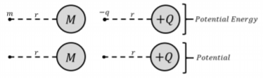
It is often useful in physics to take previously learned concepts and compare them to new ones, in this case, gravitational potential energy and electric potential energy can be compared to help understand the physical meaning of electric potential.
Suppose that an object with a large mass, \(M\), is sitting in space. Now place an object of a much smaller mass, \(m\), at any distance, \(r\), from the center of \(M\). The gravitational potential energy of the small mass is given by the following formula:
\[\begin{aligned} U_g&=\frac{GMm}{r}\end{aligned}\]
Which is very similar to the formula for electrical potential energy:
\[\begin{aligned} U(\vec r)&=\frac{kQq}{r}\end{aligned}\]
Now, if we were to remove the mass \(m\) from its position, we would no longer have an object with gravitational potential energy. However, we could still describe the gravitational potential for the point, \(r\), which would result in gravitational potential energy when any mass \(m\) is placed there. This is the gravitational equivalent to electric potential, and can be defined as:
\[\begin{aligned} V_g&=\frac{U_g}{m}\end{aligned}\]
which is also very similar to the formula for electric potential:
\[\begin{aligned} V_E&=\frac{U_E}{q}\end{aligned}\]
This comparison is illustrated in Figure \(\PageIndex{1}\).
A proton and an electron move from a region of space where the electric potential is \(20\text{V}\) to a region of space where the electric potential is \(10\text{V}\). If the electric force is the only force exerted on the particles, what can you say about their change in speed?
Solution
The two particles move from a region of space where the electric potential is \(20\text{V}\) to a region of space where the electric potential is \(10\text{V}\). The change in electric potential experienced by the particles is thus:
\[\begin{aligned} \Delta V = V_{final}-V_{initial}=(10\text{V})-(20\text{V})=-10\text{V}\end{aligned}\]
and we take the opportunity to emphasize that one should be very careful with signs when using potential. The change in potential energy of the proton, with charge \(q=+e\), is thus:
\[\begin{aligned} \Delta U_p=q\Delta V = (+e)(-10\text{V})=-10\text{eV}\end{aligned}\]
The potential energy of the proton thus decreases by \(10\text{eV}\) (which you can easily convert to Joules). Since we are told that no other force is exerted on the particle, the total mechanical energy of the particle (kinetic plus potential energies) must be constant. Thus, if the potential energy decreased, then the kinetic energy of the proton has increased by the same amount, and the proton’s speed increases.
The change in potential energy of the electron, with charge \(q=-e\), is thus:
\[\begin{aligned} \Delta U_e=q\Delta V = (-e)(-10\text{V}) = 10\text{eV}\end{aligned}\]
The potential energy of the electron thus increases by \(10\text{eV}\). Again, the mechanical energy of the electron is conserved, so that an increase in potential energy results in the same decrease in kinetic energy and the electron’s speed decreases.
Discussion
By using the electric potential, \(V\), we modelled the change in electric potential energy of a proton and an electron as they both moved from one region of space to another.
We found that when a proton moves from a region of high electric potential to a region of lower electric potential, its potential energy decreases. This is because the proton has a positive charge and a decrease in electric potential will also result in a decrease in potential energy. Since no other forces are exerted on the proton, the proton’s kinetic energy must increase. Because the potential energy of the proton decreases, the proton is moving in the same direction as the electric force, and the electric force does positive work on the proton to increase its kinetic energy.
Conversely, we found that when an electron moves from a region of high electric potential to a region of lower electric potential, its potential energy increases. This is because it has a negative charge and a decrease in electrical potential thus results in an increase in potential energy. Since no other forces are exerted on the electron, the electron’s kinetic energy must decrease, and the electron slows down. This makes sense, since the force that is exerted on an electron will be in the opposite direction from the force exerted on a proton.
Electric potential from electric field
At the beginning of Section 18.1, we determined the potential energy of a point charge, \(q\), in the presence of another point charge, \(Q\) (Figure \(\PageIndex{1}\)). This was done by calculating the work done by the Coulomb (electric) force exerted by charge \(Q\) on \(q\). We can write the same integral for the work done by the electric force on \(q\), but using the electric field, \(\vec E\), to write the force:
\[\begin{aligned} W&=\int_A^B \vec F^E\cdot d\vec r=\int_A^B q \vec E\cdot d\vec r=q \int_A^B \vec E\cdot d\vec r\end{aligned}\]
where we recognized that the charge, \(q\), is constant and can come out of the integral. The integral that is left is thus the work done by the electric field, \(\vec E\), per unit charge. In other words, this is the negative change in electric potential:
\[\begin{aligned} W=q\int_{A}^{B}\vec E\cdot d\vec r=-q\Delta V=-q[V(\vec r_{B})-V(\vec r_{A})] \end{aligned}\]
\[\therefore\Delta V=V(\vec r_{B})-V(\vec r_{A})=-\int_A^B\vec E\cdot d\vec r\]
which allows us to easily determine the change in electric potential associated with an electric field. Note that this result is general and does not require the electric field to be that of a point charge, and can be used to determine the electric potential associated with any electric field. We can also specify a function for the potential, up to an arbitrary constant, \(C\), (think definite versus indefinite integrals):
\[\begin{aligned} V(\vec r)=-\int \vec E\cdot d\vec r + C\end{aligned}\]
The relation between electric potential and electric field is analogous to the relation between electric potential energy and electric force:
\[\begin{aligned} \Delta V &=V(\vec r_B)-V(\vec r_A)=-\int_A^B \vec E\cdot d\vec r\\[4pt] \Delta U &=U(\vec r_B)-U(\vec r_A)=-\int_A^B \vec F^E\cdot d\vec r\end{aligned}\]
as the bottom equation is just \(q\) times the first equation. We can think of electric potential being to potential energy what electric field is to electric force. Electric potential and electric field are electric potential energy and electric force, per unit charge, respectively.
For a point charge, \(Q\), located at the origin, the electric field at some position, \(\vec r\), is given by Coulomb’s Law:
\[\begin{aligned} \vec E=\frac{kQ}{r^2}\hat r\end{aligned}\]
The potential difference between location \(A\) (at position \(\vec r_A\)) and location \(B\) (at position \(\vec r_B\)), as in Figure \(\PageIndex{1}\), is given by:
\[\begin{aligned} \Delta V &=- \int_A^B \vec E\cdot d\vec r= -\int_{\vec r_A}^{\vec r_B} \frac{kQ}{r^2}\hat r\cdot d\vec r=-\left(\frac{kQ}{r_B}-\frac{kQ}{r_A}\right)\end{aligned}\]
and we note that we can write a function for the electric potential, \(V(\vec r)\), at a distance \(r\) from a point charge, \(Q\), as:
\[\begin{aligned} V(\vec r)=\frac{kQ}{r}+C\end{aligned}\]
where \(C\) is an arbitrary constant. This, of course, is identical to the result that we obtained earlier, for the potential energy of a charge, \(q\), a distance, \(r\), from \(Q\).
\[\begin{aligned} U(\vec r)=qV(\vec r)=\frac{kQq}{r}+C'\end{aligned}\]
where the constant, \(C'=qC\), does not have any physical impact. Often, as is the case for gravity, one chooses the constant \(C=0\). This choice corresponds to defining potential energy to be zero at infinity. Equivalently, this corresponds to choosing infinity to be at an electric potential of \(0\text{V}\).
What causes a positively charged particle to gain speed when it is accelerated through a potential difference?:
- The particle accelerates because it loses potential energy as it moves from high to low potential.
- The particle accelerates because it loses potential energy as it moves from low to high potential
- The particle accelerates because it gains potential energy.
- The particle accelerates because it moves towards negative charges.
- Answer
What is the electric potential at the edge of a hydrogen atom (a distance of \(1\) from the proton), if one sets \(0\text{ V}\) at infinity? If an electron is located at a distance of \(1\) from the proton, how much energy is required to remove the electron; that is, how much energy is required to ionize the hydrogen atom?
Solution
We can easily calculate the electric potential, a distance of \(1\unicode{xC5}\) from a proton, since this corresponds to the potential from a point charge (with \(C=0\)):
\[\begin{aligned} V(\vec r)=\frac{kQ}{r}=\frac{(9\times 10^{9}\text{N}\cdot\text{m}^2\text{/C}^{2})(1.6\times 10^{-19}\text{C})}{(1\times 10^{-10}\text{m})}=14.4\text{V}\end{aligned}\]
We can calculate the potential energy of the electron (relative to infinity, where the potential is \(0\text{ V}\), since we chose \(C=0\)):
\[\begin{aligned} U=(-e)V=(-1.6\times 10^{-19}\text{C})(14.4\text{V})=-14.4\text{eV}=-2.3\times 10^{-18}\text{J}\end{aligned}\]
where we also expressed the potential energy in electron volts. In order to remove the electron from the hydrogen atom, we must exert a force (do work) until the electron is infinitely far from the proton. At infinity, the potential energy of the electron will be zero (by our choice of \(C=0\)). When moving the electron from the hydrogen atom to an infinite distance away, we must do positive work to counter the attractive force from the proton. The work that we must do is exactly equal to the change in potential energy of the electron (and equal to the negative of the work done by the force exerted by the proton):
\[\begin{aligned} W=\Delta U=(U_{final}-U_{initial})=(0\text{J}--2.3\times 10^{-18}\text{J})=2.3\times 10^{-18}\text{J} \end{aligned}\]
The positive work that we must do, exerting a force that is opposite to the electric force, is positive and equal to \(2.3\times 10^{-18}\text{J}\), or \(14.4\text{eV}\). If you look up the ionization energy of hydrogen, you will find that it is \(13.6\text{eV}\), so that this very simplistic model is quite accurate (we could improve the model by adjusting the proton-electron distance so that the potential is \(13.6\text{V}\)).
Discussion
In this example, we determined the electrical potential energy of an electron in a hydrogen atom, and found that it is negative, when potential energy is defined to be zero at infinity. In order to remove the electron from the atom, we must do positive work in order to increase the potential energy of the electron from a negative value to zero (the potential energy at infinity). This is analogous to the work that must be done on a satellite in a gravitationally bound orbit for it to reach escape velocity.
Two large parallel plates are separated by a distance, \(L\). The plates are oppositely charged and carry the same magnitude of charge per unit area, \(\sigma\). What is the potential difference between the two plates? Write an expression for the electric potential in the region between the two plates. Assume that the plates are large enough that you can treat them as infinite (that is, neglect what happens near the edges).
Solution
Figure \(\PageIndex{2}\) shows a diagram of the two parallel plates with surface charge on them.
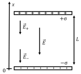
We know from the previous chapters that the electric field from the positive plate does not depend on distance from the plate and is given by:
\[\begin{aligned} \vec E_+=-\frac{\sigma}{2\epsilon_0} \hat x\end{aligned}\]
if we approximate the plate as being infinitely large. This is a reasonable approximation for most points except those near the edges of the plate, which we ignore. The electric field from the negative plate will have the same magnitude and direction, so that the total electric field, \(\vec E\), everywhere between the two parallel plates (as long as we are not near the edges) is given by:
\[\begin{aligned} \vec E=-\frac{\sigma}{\epsilon_0} \hat x\end{aligned}\]
Note that the electric field outside the region between the two plates is zero everywhere, as the field from the positive and negative plates point in opposite directions outside the plates and thus cancel (except near the edges of the plates). For example, below the negative plate, the field from the negative plate points in the positive \(x\) direction (towards the negative plate), whereas the field from the positive plate points in the positive \(x\) direction (towards the positive plate).
We can now determine the potential difference between the two plates, since we know the electric field in that region. Using the coordinate system that is shown, we calculate the potential difference between the positive plate located at \(x=L\) and the negative plate located at \(x=0\):
\[\begin{aligned} \Delta V &=V(L)-V(0)=- \int_0^L \vec E\cdot d\vec x=-\int_0^L\frac{-\sigma}{\epsilon_0} \hat x \cdot d\vec x=\frac{\sigma}{\epsilon_0}\int_0^L dx=\frac{\sigma}{\epsilon_0}L\end{aligned}\]
where we recognized that \(\hat x\) and \(d\vec x\) are parallel. It is very easy to get the wrong sign when calculating potential differences, so be careful!
Since the potential difference, \(\Delta V=V(L)-V(0)\), is positive, the plate at \(x=L\) is at a higher electric potential than the plate at \(x=0\). This makes sense, as a positive charge at rest would move from the positive plate to the negative plate, thus decreasing its potential energy, which corresponds to moving from a region of high electric potential to a region of low electric potential. Conversely, a negative charge at rest would move from the negative plate to the positive plate, decreasing its potential energy, but moving from a region of low electric potential to a region of high electric potential.
In general, if the electric field is constant, the change in potential between two points separated by a distance, \(L\), along an axis that is anti-parallel with the field (in this example, the field points in the negative \(x\) direction) is given by:
\[\begin{aligned} \Delta V =- \int_0^L \vec E\cdot d\vec x=E\int_0^L dx= EL\end{aligned}\]
Note that we can only calculate the difference in electric potential between plates, not the actual value of the potential, \(V\). If we want to define a specific value of electric potential, we need to choose a location where we define \(0\text{V}\) to be. By convention, when possible, one chooses the negative plate to be the location of \(0\text{V}\). In order to determine the electric potential anywhere between the two plates, we can calculate the potential difference between the plate at \(x=0\) (the one at \(0\text{V}\)) and some position between the plates along the \(x\) axis (\(x<L\)):
\[\begin{aligned} \Delta V &=V(x)-V(0)=-\int_0^x E \hat x \cdot d\vec x= Ex =\frac{\sigma}{\epsilon_0}x\\[4pt] \therefore V(x)&=V(0)+Ex=Ex=\frac{\sigma}{\epsilon_0}x\end{aligned}\]
where we find that the electric potential increases linearly between its value at the negative plate (\(0\text{V}\)) and its value at the positive plate (\(EL\)). Of course, we could have chosen any value of the electric potential for the negative plate, which is equivalent to choosing the value of the arbitrary constant, \(C\).
In general, we can write the electric potential in a region of constant electric field, \(\vec E=-E\hat x\), as:
\[\begin{aligned} V(x)=Ex + C\end{aligned}\]
This scenario is very similar to the gravitational force near the surface of the Earth, where the gravitational field is (almost) constant. If you choose to define zero gravitational potential energy at the surface of the Earth, then, as you move up a distance \(h\) from the ground, your gravitational potential energy increases linearly with \(h\) (\(U(h)=mgh\)). In our case, we defined zero electrical potential energy to correspond to the location of the negative plate (the negative plate is thus like the surface of the Earth, with a constant electric field pointing towards it). As a positive charge moves a distance \(h\) away from the negative plate, it gains electric potential energy, \(U(h)=qV(h)=qEh\), linearly with distance from the plate. If we release that positive charge, it will “fall” back onto the negative plate. The main difference with gravity, is that we can also have negative charges, which under gravity, would be similar to “negative masses” (it’s not a thing), which would “fall upwards” (towards the positive plate).
Discussion
In this example, we examined the electric field between two parallel plates with opposite charges on them, and saw that the field is constant and uniform between the plates and zero outside (except for a small region near the edge of the plates where the assumption of infinitely large plates breaks down). We found that the electric potential decreases linearly as a function of distance from one of the plates. Because the electric field is constant between the two plates, the electric force on a charge can be treated in a similar way as the gravitational force on a mass near the surface of the Earth. The resulting electric potential is linear in the distance from the negative plate, just as \(mgh\) is linear in \(h\), the distance to the surface of the Earth. Parallel plates are often used to accelerate charges, so they are useful to understand.
If we defined a gravitional potential, \(V(h)\), for particles a small distance, \(h\), from the surface of the Earth, it would have the form:
- \(V(h) = mgh + C\).
- \(V(h) = gh + C\).
- \(V(h) = mg + C\).
- \(V(h) = -mgh + C\).
- Answer
Electric field from electric potential
- Section 8.2 on determining force from potential energy.
- Section A2.2 on gradients.
In the previous section, we found that we could determine the electric potential (a scalar) from the electric field vector. In this section, we show how to do the reverse, and determine the electric field vector from the electric potential. Consider, first, a one-dimensional case, where the electric field, \(\vec E(x)= E(x) \hat x\), point in the \(x\) direction and depends on position, \(x\). In this one-dimensional case, the electric potential is obtained from the negative anti-derivative of the electric field:
\[\begin{aligned} V(x)=-\int \vec E(x)\cdot d\vec x=-\int E(x) dx\end{aligned}\]
The electric field must then be given by the negative of the derivative of the electric potential function:
\[\begin{aligned} \vec E(x) = -\frac{dV(x)}{dx}\hat x\end{aligned}\]
Note that we can tell from the above that the electric field must have dimensions of electric potential over distance. The most common S.I. unit used to describe the electric field is \(\text{V/m}\) (Volts per meter).
This result is very similar to that obtained in Section 8.2, where we examined how one could use the scalar potential energy, \(U(x,y,z)\), to determine the vector for the force associated with that potential energy. The same holds for the electric force, where we can determine the electric force vector, \(\vec F\), from the electric potential energy, and similarly the electric field from the electric potential. In three dimensions, if we know the electric potential energy as a function of position, \(U(\vec r)=U(x,y,z)\), then the electric force vector is given by:
\[\begin{aligned} \vec F(x,y,z) =- \nabla U=-\frac{\partial U}{\partial x}\hat x-\frac{\partial U}{\partial y}\hat y-\frac{\partial U}{\partial z}\hat z\end{aligned}\]
Similarly, but using force per unit charge (i.e. electric field) and potential energy per unit charge (i.e. electric potential), we find:
\[\begin{aligned} \vec E(x,y,z) = -\nabla V =-\frac{\partial V}{\partial x}\hat x-\frac{\partial V}{\partial y}\hat y-\frac{\partial V}{\partial z}\hat z\end{aligned}\]
where, as you recall, \(\nabla V\), is called the gradient of the scalar field, \(V(x,y,z)\). The gradient is a vector that points in the direction of maximal increase of the value of \(V(x,y,z)\). For a positive charge, this corresponds to the direction of maximal increase in potential energy. A positive charge will experience a force in the opposite direction (in the direction where the potential energy decreases the fastest), and the electric field is thus in the opposite direction from the gradient of the electric potential.
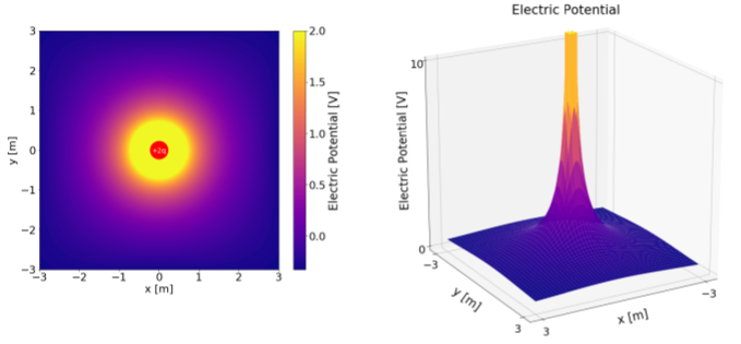
Equipotential surfaces
We can visualize electric potential in several ways, since it is a scalar field (it has a single value that can differ everywhere in space). Figure \(\PageIndex{3}\) shows the electric potential near a positive charge, \(+Q\), where one has chosen \(0\text{V}\) to be located at infinity. The right panel shows the electric potential as a “surface plot”, where the vertical direction is the value of the electric potential. The left panel shows a “heat map” of the electric potential, where the color corresponds to the value of the electric potential.
The most common way to visualize the electric potential is to draw “contour lines”, similar to how one draws contour lines on a geographical map. On a geographical map, contours correspond to lines of constant altitude, which are also lines of constant gravitational potential energy. Similarly, we can draw lines of constant electric potential to visualize the electric potential. Lines of constant potential are called “equipotential lines”. In general, in three dimensions, regions of constant electric potential can be surfaces or volumes, called “equipotential surfaces/volumes”. In Example 18.2.3 (with the parallel plates) each of the plates forms an equipotential surface (e.g. the electric potential was fixed to \(0\text{V}\) everywhere on the negative plate).
Recall that, at some point in space, the electric field vector always points in the opposite direction of the gradient of the electric potential. Namely, the electric field points in the direction in which the electric potential decreases the fastest. That direction must be perpendicular to the direction in which the electric potential does not change; in other words, the electric field vector is always perpendicular to equipotential lines/surfaces. More intuitively, one can think about a charge moving along an equipotential. By definition, the electric potential energy of the charge does not change if its moves along an equipotential. As a result, the electric force/field cannot do any work on the charge, and must thus be perpendicular to the path of the charge (which we chose to be an equipotential).
Conducting materials are always equipotential surfaces (or volumes) if charges are not moving inside the conductor. The electric field inside a conductor is always zero (in electrostatics, when charges are not moving), and thus, a charge moving through a conductor experiences no electric force and its electrical potential energy will be constant; in other words, the entire conductor is an equipotential. Similarly, because the electric field must always be perpendicular to an equipotential, electric field lines are always perpendicular to the surface of a conductor (in electrostatics).
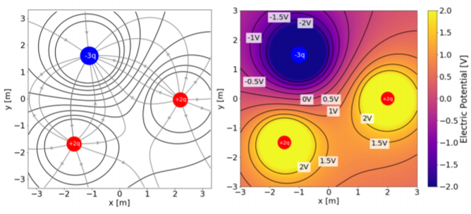
In order to draw equipotential lines, one can start by drawing electric field lines, and then draw (closed) contour lines that are everywhere perpendicular to the electric field lines. This is illustrated in Figure \(\PageIndex{4}\).
In general, it is preferable to draw equipotential lines that are separated by equal increments in electric potential (just as on a geographical map, the contour lines correspond to constant increments in altitude). This requires knowing a functional form for the electric potential. For example, the equipotential lines for a point charge located at the origin consist in concentric circles centerd at the origin (in three dimensions, this results in concentric spherical equipotential surfaces). If we define \(0\text{V}\) to be at infinity, the electric potential is given by:
\[\begin{aligned} V(r)=\frac{kQ}{r}\end{aligned}\]
In order to draw equipotential lines every, say, \(10\text{V}\), the radii of the corresponding equipotential circles, for \(V=10\text{V}\), \(V=20\text{V}\), \(V=30\text{V}\), etc., are given by:
\[\begin{aligned} r&=\frac{kQ}{V}\\[4pt] r_{10V}&=\frac{kQ}{(10\text{V})}\quad r_{20V}=\frac{kQ}{(20\text{V})}\quad r_{30V}=\frac{kQ}{(30\text{V})}\quad \dots\end{aligned}\]