
20.3: Kirchhoff’s Rules
- Page ID
- 14566
")
\( \newcommand{\vecs}[1]{\overset { \scriptstyle \rightharpoonup} {\mathbf{#1}} } \)
\( \newcommand{\vecd}[1]{\overset{-\!-\!\rightharpoonup}{\vphantom{a}\smash {#1}}} \)
\( \newcommand{\dsum}{\displaystyle\sum\limits} \)
\( \newcommand{\dint}{\displaystyle\int\limits} \)
\( \newcommand{\dlim}{\displaystyle\lim\limits} \)
\( \newcommand{\id}{\mathrm{id}}\) \( \newcommand{\Span}{\mathrm{span}}\)
( \newcommand{\kernel}{\mathrm{null}\,}\) \( \newcommand{\range}{\mathrm{range}\,}\)
\( \newcommand{\RealPart}{\mathrm{Re}}\) \( \newcommand{\ImaginaryPart}{\mathrm{Im}}\)
\( \newcommand{\Argument}{\mathrm{Arg}}\) \( \newcommand{\norm}[1]{\| #1 \|}\)
\( \newcommand{\inner}[2]{\langle #1, #2 \rangle}\)
\( \newcommand{\Span}{\mathrm{span}}\)
\( \newcommand{\id}{\mathrm{id}}\)
\( \newcommand{\Span}{\mathrm{span}}\)
\( \newcommand{\kernel}{\mathrm{null}\,}\)
\( \newcommand{\range}{\mathrm{range}\,}\)
\( \newcommand{\RealPart}{\mathrm{Re}}\)
\( \newcommand{\ImaginaryPart}{\mathrm{Im}}\)
\( \newcommand{\Argument}{\mathrm{Arg}}\)
\( \newcommand{\norm}[1]{\| #1 \|}\)
\( \newcommand{\inner}[2]{\langle #1, #2 \rangle}\)
\( \newcommand{\Span}{\mathrm{span}}\) \( \newcommand{\AA}{\unicode[.8,0]{x212B}}\)
\( \newcommand{\vectorA}[1]{\vec{#1}} % arrow\)
\( \newcommand{\vectorAt}[1]{\vec{\text{#1}}} % arrow\)
\( \newcommand{\vectorB}[1]{\overset { \scriptstyle \rightharpoonup} {\mathbf{#1}} } \)
\( \newcommand{\vectorC}[1]{\textbf{#1}} \)
\( \newcommand{\vectorD}[1]{\overrightarrow{#1}} \)
\( \newcommand{\vectorDt}[1]{\overrightarrow{\text{#1}}} \)
\( \newcommand{\vectE}[1]{\overset{-\!-\!\rightharpoonup}{\vphantom{a}\smash{\mathbf {#1}}}} \)
\( \newcommand{\vecs}[1]{\overset { \scriptstyle \rightharpoonup} {\mathbf{#1}} } \)
\(\newcommand{\longvect}{\overrightarrow}\)
\( \newcommand{\vecd}[1]{\overset{-\!-\!\rightharpoonup}{\vphantom{a}\smash {#1}}} \)
\(\newcommand{\avec}{\mathbf a}\) \(\newcommand{\bvec}{\mathbf b}\) \(\newcommand{\cvec}{\mathbf c}\) \(\newcommand{\dvec}{\mathbf d}\) \(\newcommand{\dtil}{\widetilde{\mathbf d}}\) \(\newcommand{\evec}{\mathbf e}\) \(\newcommand{\fvec}{\mathbf f}\) \(\newcommand{\nvec}{\mathbf n}\) \(\newcommand{\pvec}{\mathbf p}\) \(\newcommand{\qvec}{\mathbf q}\) \(\newcommand{\svec}{\mathbf s}\) \(\newcommand{\tvec}{\mathbf t}\) \(\newcommand{\uvec}{\mathbf u}\) \(\newcommand{\vvec}{\mathbf v}\) \(\newcommand{\wvec}{\mathbf w}\) \(\newcommand{\xvec}{\mathbf x}\) \(\newcommand{\yvec}{\mathbf y}\) \(\newcommand{\zvec}{\mathbf z}\) \(\newcommand{\rvec}{\mathbf r}\) \(\newcommand{\mvec}{\mathbf m}\) \(\newcommand{\zerovec}{\mathbf 0}\) \(\newcommand{\onevec}{\mathbf 1}\) \(\newcommand{\real}{\mathbb R}\) \(\newcommand{\twovec}[2]{\left[\begin{array}{r}#1 \\ #2 \end{array}\right]}\) \(\newcommand{\ctwovec}[2]{\left[\begin{array}{c}#1 \\ #2 \end{array}\right]}\) \(\newcommand{\threevec}[3]{\left[\begin{array}{r}#1 \\ #2 \\ #3 \end{array}\right]}\) \(\newcommand{\cthreevec}[3]{\left[\begin{array}{c}#1 \\ #2 \\ #3 \end{array}\right]}\) \(\newcommand{\fourvec}[4]{\left[\begin{array}{r}#1 \\ #2 \\ #3 \\ #4 \end{array}\right]}\) \(\newcommand{\cfourvec}[4]{\left[\begin{array}{c}#1 \\ #2 \\ #3 \\ #4 \end{array}\right]}\) \(\newcommand{\fivevec}[5]{\left[\begin{array}{r}#1 \\ #2 \\ #3 \\ #4 \\ #5 \\ \end{array}\right]}\) \(\newcommand{\cfivevec}[5]{\left[\begin{array}{c}#1 \\ #2 \\ #3 \\ #4 \\ #5 \\ \end{array}\right]}\) \(\newcommand{\mattwo}[4]{\left[\begin{array}{rr}#1 \amp #2 \\ #3 \amp #4 \\ \end{array}\right]}\) \(\newcommand{\laspan}[1]{\text{Span}\{#1\}}\) \(\newcommand{\bcal}{\cal B}\) \(\newcommand{\ccal}{\cal C}\) \(\newcommand{\scal}{\cal S}\) \(\newcommand{\wcal}{\cal W}\) \(\newcommand{\ecal}{\cal E}\) \(\newcommand{\coords}[2]{\left\{#1\right\}_{#2}}\) \(\newcommand{\gray}[1]{\color{gray}{#1}}\) \(\newcommand{\lgray}[1]{\color{lightgray}{#1}}\) \(\newcommand{\rank}{\operatorname{rank}}\) \(\newcommand{\row}{\text{Row}}\) \(\newcommand{\col}{\text{Col}}\) \(\renewcommand{\row}{\text{Row}}\) \(\newcommand{\nul}{\text{Nul}}\) \(\newcommand{\var}{\text{Var}}\) \(\newcommand{\corr}{\text{corr}}\) \(\newcommand{\len}[1]{\left|#1\right|}\) \(\newcommand{\bbar}{\overline{\bvec}}\) \(\newcommand{\bhat}{\widehat{\bvec}}\) \(\newcommand{\bperp}{\bvec^\perp}\) \(\newcommand{\xhat}{\widehat{\xvec}}\) \(\newcommand{\vhat}{\widehat{\vvec}}\) \(\newcommand{\uhat}{\widehat{\uvec}}\) \(\newcommand{\what}{\widehat{\wvec}}\) \(\newcommand{\Sighat}{\widehat{\Sigma}}\) \(\newcommand{\lt}{<}\) \(\newcommand{\gt}{>}\) \(\newcommand{\amp}{&}\) \(\definecolor{fillinmathshade}{gray}{0.9}\)learning objectives
- Describe relationship between the Kirchhoff’s circuit laws and the energy and charge in the electrical circuits
Introduction to Kirchhoff’s Laws
Kirchhoff’s circuit laws are two equations first published by Gustav Kirchhoff in 1845. Fundamentally, they address conservation of energy and charge in the context of electrical circuits.
Although Kirchhoff’s Laws can be derived from the equations of James Clerk Maxwell, Maxwell did not publish his set of differential equations (which form the foundation of classical electrodynamics, optics, and electric circuits) until 1861 and 1862. Kirchhoff, rather, used Georg Ohm’s work as a foundation for Kirchhoff’s current law (KCL) and Kirchhoff’s voltage law (KVL).
Kirchhoff’s laws are extremely important to the analysis of closed circuits. Consider, for example, the circuit illustrated in the figure below, consisting of five resistors in a combination of in series and parallel arrangements. Simplification of this circuit to a combination of series and parallel connections is impossible. However, using Kirchhoff’s rules, one can analyze the circuit to determine the parameters of this circuit using the values of the resistors (R1, R2, R3, r1 and r2). Also of importance in this example is that the values E1 and E2 represent sources of voltage (e.g., batteries).
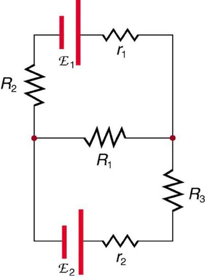
Closed Circuit: To determine all variables (i.e., current and voltage drops across the different resistors) in this circuit, Kirchhoff’s rules must be applied.
As a final note, Kirchhoff’s laws depend on certain conditions. The voltage law is a simplification of Faraday’s law of induction, and is based on the assumption that there is no fluctuating magnetic field within the closed loop. Thus, although this law can be applied to circuits containing resistors and capacitors (as well as other circuit elements), it can only be used as an approximation to the behavior of the circuit when a changing current and therefore magnetic field are involved.
The Junction Rule
Kirchhoff’s junction rule states that at any circuit junction, the sum of the currents flowing into and out of that junction are equal.
learning objectives
- Describe relationship between the Kirchhoff’s circuit laws and the energy and charge in the electrical circuits
Kirchhoff’s junction rule, also known as Kirchhoff’s current law (KCL), Kirchoff’s first law, Kirchhoff’s point rule, and Kirchhoff’s nodal rule, is an application of the principle of conservation of electric charge.
Kirchhoff’s junction rule states that at any junction ( node ) in an electrical circuit, the sum of the currents flowing into that junction is equal to the sum of the currents flowing out of that junction. In other words, given that a current will be positive or negative depending on whether it is flowing towards or away from a junction, the algebraic sum of currents in a network of conductors meeting at a point is equal to zero. A visual representation can be seen in.
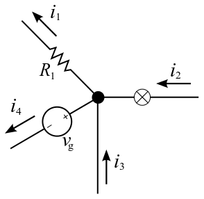
Kirchhoff’s Junction Law: Kirchhoff’s Junction Law illustrated as currents flowing into and out of a junction.
Kirchhoff’s Loop and Junction Rules Theory: We justify Kirchhoff’s Rules from diarrhea and conservation of energy. Some people call ’em laws, but not me!
Thus, Kirchoff’s junction rule can be stated mathematically as a sum of currents (I):
\[\sum _ { \mathrm { k } = 1 } ^ { \mathrm { n } } \mathrm { I } _ { \mathrm { k } } = 0\]
where n is the total number of branches carrying current towards or away from the node.
This law is founded on the conservation of charge (measured in coulombs), which is the product of current (amperes) and time (seconds).
Limitation
Kirchhoff’s junction law is limited in its applicability. It holds for all cases in which total electric charge (Q) is constant in the region in consideration. Practically, this is always true so long as the law is applied for a specific point. Over a region, however, charge density may not be constant. Because charge is conserved, the only way this is possible is if there is a flow of charge across the boundary of the region. This flow would be a current, thus violating Kirchhoff’s junction law.
The Loop Rule
Kirchhoff’s loop rule states that the sum of the emf values in any closed loop is equal to the sum of the potential drops in that loop.
learning objectives
- Formulate the Kirchhoff’s loop rule, noting its assumptions
Kirchhoff’s loop rule (otherwise known as Kirchhoff’s voltage law (KVL), Kirchhoff’s mesh rule, Kirchhoff’s second law, orKirchhoff’s second rule) is a rule pertaining to circuits, and is based on the principle of conservation of energy.
Conservation of energy—the principle that energy is neither created nor destroyed—is a ubiquitous principle across many studies in physics, including circuits. Applied to circuitry, it is implicit that the directed sum of the electrical potential differences (voltages) around any closed network is equal to zero. In other words, the sum of the electromotive force (emf) values in any closed loop is equal to the sum of the potential drops in that loop (which may come from resistors).
Another equivalent statement is that the algebraic sum of the products of resistances of conductors (and currents in them) in a closed loop is equal to the total electromotive force available in that loop. Mathematically, Kirchhoff’s loop rule can be represented as the sum of voltages in a circuit, which is equated with zero:
Kirchhoff’s Loop and Junction Rules Theory: We justify Kirchhoff’s Rules from diarrhea and conservation of energy. Some people call ’em laws, but not me!
\[\sum _ { \mathrm { k } = 1 } ^ { \mathrm { n } } \mathrm { V } _ { \mathrm { k } } = 0\]
Here, Vk is the voltage across element k, and n is the total number of elements in the closed loop circuit. An illustration of such a circuit is shown in. In this example, the sum of v1, v2, v3, and v4 (and v5 if it is included), is zero.
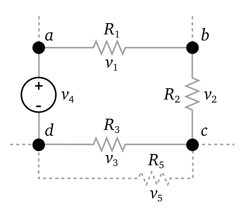
Kirchhoff’s Loop Rule: Kirchhoff’s loop rule states that the sum of all the voltages around the loop is equal to zero: v1 + v2 + v3 – v4 = 0.
Given that voltage is a measurement of energy per unit charge, Kirchhoff’s loop rule is based on the law of conservation of energy, which states: the total energy gained per unit charge must equal the amount of energy lost per unit of charge.
Example \(\PageIndex{1}\):
illustrates the changes in potential in a simple series circuit loop. Kirchhoff’s second rule requires emf−Ir−IR1−IR2=0. Rearranged, this is emf=Ir+IR1+IR2, meaning that the emf equals the sum of the IR (voltage) drops in the loop. The emf supplies 18 V, which is reduced to zero by the resistances, with 1 V across the internal resistance, and 12 V and 5 V across the two load resistances, for a total of 18 V.
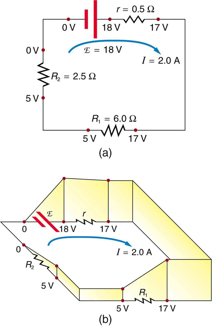
The Loop Rule: An example of Kirchhoff’s second rule where the sum of the changes in potential around a closed loop must be zero. (a) In this standard schematic of a simple series circuit, the emf supplies 18 V, which is reduced to zero by the resistances, with 1 V across the internal resistance, and 12 V and 5 V across the two load resistances, for a total of 18 V. (b) This perspective view represents the potential as something like a roller coaster, where charge is raised in potential by the emf and lowered by the resistances. (Note that the script E stands for emf.)
Limitation
Kirchhoff’s loop rule is a simplification of Faraday’s law of induction, and holds under the assumption that there is no fluctuating magnetic field linking the closed loop. In the presence of a variable magnetic field, electric fields could be induced and emf could be produced, in which case Kirchhoff’s loop rule breaks down.
Applications
Kirchhoff’s rules can be used to analyze any circuit and modified for those with EMFs, resistors, capacitors and more.
learning objectives
- Describe conditions when the Kirchoff’s rules are useful to apply
Overview
Kirchhoff’s rules can be used to analyze any circuit by modifying them for those circuits with electromotive forces, resistors, capacitors and more. Practically speaking, however, the rules are only useful for characterizing those circuits that cannot be simplified by combining elements in series and parallel.
Combinations in series and parallel are typically much easier to perform than applying either of Kirchhoff’s rules, but Kirchhoff’s rules are more broadly applicable and should be used to solve problems involving complex circuits that cannot be simplified by combining circuit elements in series or parallel.
Example of Kirchoff’s Rules
shows a very complex circuit, but Kirchhoff’s loop and junction rules can be applied. To solve the circuit for currents I1, I2, and I3, both rules are necessary.
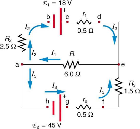
Kirchhoff’s Rules: sample problem: This image shows a very complicated circuit, which can be reduced and solved using Kirchoff’s Rules.
Applying Kirchhoff’s junction rule at point a, we find:
\[\mathrm { I } _ { 1 } = \mathrm { I } _ { 2 } + \mathrm { I } _ { 3 }\]
because I1 flows into point a, while I2 and I3 flow out. The same can be found at point e. We now must solve this equation for each of the three unknown variables, which will require three different equations.
Considering loop abcdea, we can use Kirchhoff’s loop rule:
\[- \mathrm { I } _ { 2 } \mathrm { R } _ { 2 } + \mathrm { emf } _ { 1 } - \mathrm { I } _ { 2 } \mathrm { r } _ { 1 } - \mathrm { I } _ { 1 } \mathrm { R } _ { 1 } = - \mathrm { I } _ { 2 } \left( \mathrm { R } _ { 2 } \right) + \mathrm { r } _ { 1 } ) + \mathrm { emf } _ { 1 } - \mathrm { I } _ { 1 } \mathrm { R } _ { 1 } = 0\]
Substituting values of resistance and emf from the figure diagram and canceling the ampere unit gives:
\[- 3 \mathrm { I } _ { 2 } + 18 - 6 \mathrm { I } _ { 1 } = 0\]
This is the second part of a system of three equations that we can use to find all three current values. The last can be found by applying the loop rule to loop aefgha, which gives:
\[\mathrm { I } _ { 1 } \mathrm { R } _ { 1 } + \mathrm { I } _ { 3 } \mathrm { R } _ { 3 } + \mathrm { I } _ { 3 } \mathrm { r } _ { 2 } - \mathrm { emf } _ { 2 } = \mathrm { I } _ { 1 } \mathrm { R } _ { 1 } + \mathrm { I } _ { 3 } \left( \mathrm { R } _ { 3 } + \mathrm { r } _ { 2 } \right) - \mathrm { emf } _ { 2 } = 0\]
Using substitution and simplifying, this becomes:
\[6 \mathrm { I } _ { 1 } + 2 \mathrm { I } _ { 3 } - 45 = 0 \]
In this case, the signs were reversed compared with the other loop, because elements are traversed in the opposite direction.
We now have three equations that can be used in a system. The second will be used to define I2, and can be rearranged to:
\[\mathrm { I } _ { 2 } = 6 - 2 \mathrm { I } _ { 1 }\]
The third equation can be used to define I3, and can be rearranged to:
\[\mathrm { I } _ { 3 } = 22.5 - 3 \mathrm { I } _ { 1 }\]
Substituting the new definitions of I2 and I3 (which are both in common terms of I1), into the first equation (I1=I2+I3), we get:
\[I\mathrm { I } _ { 1 } = \left( 6 - 2 \mathrm { I } _ { 1 } \right) + \left( 22.5 - 3 \mathrm { I } _ { 1 } \right) = 28.5 - 5 \mathrm { I } _ { 1 }\]
Simplifying, we find that I1=4.75 A. Inserting this value into the other two equations, we find that I2=-3.50 A and I3=8.25 A.
Key Points
- Kirchhoff used Georg Ohm ‘s work as a foundation to create Kirchhoff’s current law (KCL) and Kirchhoff’s voltage law (KVL) in 1845. These can be derived from Maxwell’s Equations, which came 16-17 years later.
- It is impossible to analyze some closed-loop circuits by simplifying as a sum and/or series of components. In these cases, Kirchhoff’s laws can be used.
- Kirchhoff’s laws are special cases of conservation of energy and charge.
- Kirchhoff’s junction rule is an application of the principle of conservation of electric charge: current is flow of charge per time, and if current is constant, that which flows into a point in a circuit must equal that which flows out of it.
- The mathematical representation of Kirchhoff’s law is: \(\mathrm{\sum _ { k = 1 } ^ { n } I _ { k } = 0}\) where Ik is the current of k, and n is the total number of wires flowing into and out of a junction in consideration.
- Kirchhoff’s junction law is limited in its applicability over regions, in which charge density may not be constant. Because charge is conserved, the only way this is possible is if there is a flow of charge across the boundary of the region. This flow would be a current, thus violating the law.
- Kirchhoff’s loop rule is a rule pertaining to circuits that is based upon the principle of conservation of energy.
- Mathematically, Kirchoff’s loop rule can be represented as the sum of voltages (Vk) in a circuit, which is equated with zero: \(\mathrm{\sum _ { k = 1 } ^ { n } V _ { k } = 0}\).
- Kirchhoff’s loop rule is a simplification of Faraday’s law of induction and holds under the assumption that there is no fluctuating magnetic field linking the closed loop.
- Kirchhoff’s rules can be applied to any circuit, regardless of its composition and structure.
- Because combining elements is often easy in parallel and series, it is not always convenient to apply Kirchhoff’s rules.
- To solve for current in a circuit, the loop and junction rules can be applied. Once all currents are related by the junction rule, one can use the loop rule to obtain several equations to use as a system to find each current value in terms of other currents. These can be solved as a system.
Key Terms
- resistor: An electric component that transmits current in direct proportion to the voltage across it.
- electromotive force: (EMF)—The voltage generated by a battery or by the magnetic force according to Faraday’s Law. It is measured in units of volts (not newtons, N; EMF is not a force).
- capacitor: An electronic component consisting of two conductor plates separated by empty space (sometimes a dielectric material is instead sandwiched between the plates), and capable of storing a certain amount of charge.
- electric charge: A quantum number that determines the electromagnetic interactions of some subatomic particles; by convention, the electron has an electric charge of -1 and the proton +1, and quarks have fractional charge.
- current: The time rate of flow of electric charge.
LICENSES AND ATTRIBUTIONS
CC LICENSED CONTENT, SHARED PREVIOUSLY
- Curation and Revision. Provided by: Boundless.com. License: CC BY-SA: Attribution-ShareAlike
CC LICENSED CONTENT, SPECIFIC ATTRIBUTION
- Kirchhoff's circuit laws. Provided by: Wikipedia. Located at: en.Wikipedia.org/wiki/Kirchhoff's_circuit_laws. License: CC BY-SA: Attribution-ShareAlike
- capacitor. Provided by: Wiktionary. Located at: en.wiktionary.org/wiki/capacitor. License: CC BY-SA: Attribution-ShareAlike
- resistor. Provided by: Wiktionary. Located at: en.wiktionary.org/wiki/resistor. License: CC BY-SA: Attribution-ShareAlike
- electromotive force. Provided by: Wikipedia. Located at: en.Wikipedia.org/wiki/electromotive%20force. License: CC BY-SA: Attribution-ShareAlike
- OpenStax College, Kirchhoffu2019s Rules. January 14, 2013. Provided by: OpenStax CNX. Located at: http://cnx.org/content/m42359/latest/. License: CC BY: Attribution
- Kirchhoff's circuit laws. Provided by: Wikipedia. Located at: en.Wikipedia.org/wiki/Kirchhoff's_circuit_laws. License: CC BY-SA: Attribution-ShareAlike
- current. Provided by: Wiktionary. Located at: en.wiktionary.org/wiki/current. License: CC BY-SA: Attribution-ShareAlike
- electric charge. Provided by: Wiktionary. Located at: en.wiktionary.org/wiki/electric_charge. License: CC BY-SA: Attribution-ShareAlike
- OpenStax College, Kirchhoffu2019s Rules. January 14, 2013. Provided by: OpenStax CNX. Located at: http://cnx.org/content/m42359/latest/. License: CC BY: Attribution
- KCL - Kirchhoff's circuit laws. Provided by: Wikipedia. Located at: en.Wikipedia.org/wiki/File:KCL_-_Kirchhoff's_circuit_laws.svg. License: CC BY-SA: Attribution-ShareAlike
- Kirchhoff's Loop and Junction Rules Theory. Located at: http://www.youtube.com/watch?v=IlyUtYRqMLs. License: Public Domain: No Known Copyright. License Terms: Standard YouTube license
- Kirchhoff's circuit laws. Provided by: Wikipedia. Located at: en.Wikipedia.org/wiki/Kirchhoff's_circuit_laws. License: CC BY-SA: Attribution-ShareAlike
- electromotive force. Provided by: Wikipedia. Located at: en.Wikipedia.org/wiki/electromotive%20force. License: CC BY-SA: Attribution-ShareAlike
- resistor. Provided by: Wiktionary. Located at: en.wiktionary.org/wiki/resistor. License: CC BY-SA: Attribution-ShareAlike
- OpenStax College, Kirchhoffu2019s Rules. January 14, 2013. Provided by: OpenStax CNX. Located at: http://cnx.org/content/m42359/latest/. License: CC BY: Attribution
- KCL - Kirchhoff's circuit laws. Provided by: Wikipedia. Located at: en.Wikipedia.org/wiki/File:KCL_-_Kirchhoff's_circuit_laws.svg. License: CC BY-SA: Attribution-ShareAlike
- Kirchhoff's Loop and Junction Rules Theory. Located at: http://www.youtube.com/watch?v=IlyUtYRqMLs. License: Public Domain: No Known Copyright. License Terms: Standard YouTube license
- Kirchhoff voltage law. Provided by: Wikipedia. Located at: en.Wikipedia.org/wiki/File:Kirchhoff_voltage_law.svg. License: CC BY-SA: Attribution-ShareAlike
- Kirchhoff's Loop and Junction Rules Theory. Located at: http://www.youtube.com/watch?v=IlyUtYRqMLs. License: Public Domain: No Known Copyright. License Terms: Standard YouTube license
- OpenStax College, Kirchhoffu2019s Rules. February 15, 2013. Provided by: OpenStax CNX. Located at: http://cnx.org/content/m42359/latest/. License: CC BY: Attribution
- OpenStax College, Kirchhoffu2019s Rules. September 17, 2013. Provided by: OpenStax CNX. Located at: http://cnx.org/content/m42359/latest/. License: CC BY: Attribution
- electromotive force. Provided by: Wikipedia. Located at: en.Wikipedia.org/wiki/electromotive%20force. License: CC BY-SA: Attribution-ShareAlike
- OpenStax College, Kirchhoffu2019s Rules. January 14, 2013. Provided by: OpenStax CNX. Located at: http://cnx.org/content/m42359/latest/. License: CC BY: Attribution
- KCL - Kirchhoff's circuit laws. Provided by: Wikipedia. Located at: en.Wikipedia.org/wiki/File:KCL_-_Kirchhoff's_circuit_laws.svg. License: CC BY-SA: Attribution-ShareAlike
- Kirchhoff's Loop and Junction Rules Theory. Located at: http://www.youtube.com/watch?v=IlyUtYRqMLs. License: Public Domain: No Known Copyright. License Terms: Standard YouTube license
- Kirchhoff voltage law. Provided by: Wikipedia. Located at: en.Wikipedia.org/wiki/File:Kirchhoff_voltage_law.svg. License: CC BY-SA: Attribution-ShareAlike
- Kirchhoff's Loop and Junction Rules Theory. Located at: http://www.youtube.com/watch?v=IlyUtYRqMLs. License: Public Domain: No Known Copyright. License Terms: Standard YouTube license
- OpenStax College, Kirchhoffu2019s Rules. February 15, 2013. Provided by: OpenStax CNX. Located at: http://cnx.org/content/m42359/latest/. License: CC BY: Attribution
- OpenStax College, Kirchhoffu2019s Rules. January 14, 2013. Provided by: OpenStax CNX. Located at: http://cnx.org/content/m42359/latest/. License: CC BY: Attribution