6.1: Concepts and Principles

Imagine an object at rest at its equilibrium position, for example, a pendulum hanging straight downward, an object dangling from an elastic cord, or a diving board perfectly horizontal. When these objects are displaced from equilibrium, and released, they return toward their equilibrium position. However, their trip back toward equilibrium involves repeated oscillations about the location of equilibrium. If the initial disturbance is small enough, all of these systems exhibit mathematically similar behavior. This chapter explores the similarities in their oscillatory behavior.

We will analyze in detail the motion of a common oscillator; a mass attached to the end of a spring. We will investigate the resulting motion both without including the effects of friction (undamped) and including the effects of friction (damped). You should then be able to generalize these results for arbitrary oscillatory systems.

Undamped Spring-Mass Oscillator

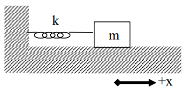
One of the simplest systems exhibiting oscillatory behavior is the spring-mass system pictured at left. A linear spring of constant k is attached to a mass m. The equilibrium position of the spring-mass system is denoted as the origin of a coordinate system.

Now imagine the block is pulled to the right and let go. Hopefully you can convince yourself that the block will oscillate back and forth. Let’s apply Newton’s Second Law at the instant the mass is at an arbitrary position, x. The only force acting on the mass in the x-direction is the force of the spring.

\[\begin{aligned}
&\Sigma F=m a \\
&F_{\text {spring }}=m a \\
&-k s=m a
\end{aligned} \nonumber\]

Because of our choice of coordinate system, the stretch of the spring (s) is exactly equal to the location of the block (x). Therefore,

\[-k x=m a \nonumber\]

Note that when the block is at a positive position, the force of the spring is in the negative direction and when the block is at a negative position, the force of the spring is in the positive direction. Thus, the force of the spring always acts to return the block to equilibrium.

Rearranging gives

\[\begin{aligned}
&-\frac{k}{m} x=a \\
&-\frac{k}{m} x=\frac{d^{2} x}{d t^{2}}
\end{aligned} \nonumber\]

and defining a constant, \(\omega^{2}\), as

\[\omega^{2}=\frac{k}{m} \nonumber\]

(Granted, it seems pretty silly to define \(\frac{k}{m}\) as the square of a constant, but just play along. You may also find it frustrating to learn that this “omega” is not an angular velocity. The block doesn’t even have an angular velocity!)

yields,

\[-\omega^{2} x=\frac{d^{2} x}{d t^{2}} \nonumber\]

Therefore, the position function for the block must have a second time derivative equal to the product of (\(-\omega^{2}\)) and itself. The only functions whose second time derivative is equal to the product of a negative constant and itself are the sine and the cosine functions. Therefore, a solution to this differential equation¹

\[-\omega^{2} x=\frac{d^{2} x}{d t^{2}} \nonumber\]

can be written:

\[x(t)=A \cos (\omega t+\phi) \nonumber\]

or equivalently with the sine function, where A and \(\phi\) are arbitrary constants.²

• A is the amplitude of the oscillation. The amplitude is the maximum displacement of the object from equilibrium.
• \(\boldsymbol{\phi}\) is the phase angle. The phase angle is used to adjust the function forward or backward in time. For example, if the particle is at the origin at t = 0 s, \(\phi\) must equal \(+\pi / 2\) or \(-\pi / 2\) to ensure that the cosine function evaluates to zero at t = 0 s. If the particle is at its maximum position at t = 0 s, then the phase angle must be zero or \(\pi\) to ensure that the cosine function evaluates to +1 or -1 at t = 0 s.
• \(\boldsymbol{\omega}\) is the angular frequency of the oscillation.³

Note

¹ A differential equation is an equation involving a function and its derivative(s).

² To prove to yourself that this is indeed the solution to the equation, you should substitute the function, x(t), into the left side of the equation and the second derivative of x(t) into the right side. This will verify that the two sides of the equation are equal. In addition to mathematically verifying this solution, you should verify the solution physically by sketching a graph of the motion that you know would result if the block were displaced to the right and comparing that sketch to a sketch of the function.

³ Again, note that \(\omega\) is not the angular velocity. The block is not rotating; it does not have an angular velocity

Note that the cosine function repeats itself when its argument increases by 2\(\pi\). Thus, when

\[\Delta(\omega t+\phi)=2 \pi \nonumber\]

the function repeats. Since \(\omega\) and \(\phi\) are constant,

\[\Delta(\omega t+\phi)=\omega \Delta t \nonumber\]

Therefore, the time interval when

\[\omega \Delta t=2 \pi \nonumber\]

is the time interval for one complete cycle of the oscillatory motion. The time for one complete cycle of the motion is termed the period, T. Thus,

\[T=\frac{2 \pi}{\omega} \nonumber\]

Therefore, the physical significance of the angular frequency is that it is inversely proportional to the period.

Substituting in the definition of \(\omega\):

\[\omega=\sqrt{\frac{k}{m}} \nonumber\]

yields

\[T=2 \pi \sqrt{\frac{m}{k}} \nonumber\]

In summary, a mass attached to a spring will oscillate about its equilibrium position with a position function given by:

\[x(t)=A \cos (\omega t+\phi) \nonumber\]

This function repeats with a period of

\[T=2 \pi \sqrt{\frac{m}{k}} \nonumber\]

Since we have an understanding of the position of the oscillating object as a function of time, we have a complete kinematic description of the motion.

Damped Spring-Mass Oscillator

Imagine the same scenario investigated above, a block displaced to the right of equilibrium by a distance x. However, let’s try to incorporate the frictional forces acting on the block. Let’s imagine that the primary frictional force acting on the block is proportional to the block’s velocity.⁴

\[\begin{aligned}
&F_{\text {friction }}=-b v \\
&F_{\text {friction }}=-b \frac{d x}{d t}
\end{aligned} \nonumber\]

The negative sign implies that the direction of the frictional force is opposite to the direction of the block’s velocity. The constant, b, is termed the drag coefficient.

Applying Newton’s Second Law now yields:

\[\begin{aligned}
&\Sigma F=m a \\
&-k x-b \frac{d x}{d t}=m \frac{d^{2} x}{d t^{2}}
\end{aligned} \nonumber\]

This is obviously a much more complicated differential equation to solve. Let’s see if we can make any headway by thinking physically about the equation.

I would expect a solution that still oscillates like a cosine function, but with amplitude that gradually decreases due to friction. Therefore, a possible solution is

\[x(t)=A e^{-\alpha t} \cos \left(\omega^{\prime} t+\phi\right) \nonumber\]

where A and \(\phi\) are arbitrary constants. If you substitute this function and its derivatives into the above equation, you will see that it is a solution of the differential equation only if:

\[\alpha=\frac{b}{2 m} \nonumber\]

and

\[\omega^{\prime}=\sqrt{\omega^{2}-\alpha^{2}} \nonumber\]

Although this result was produced in a whirlwind of (unseen) mathematics, it does have a number of physical properties that make it plausible. For one, if there is no damping (b = 0), then \(\alpha=0\), \(\omega^{\prime}=\omega\), and x(t) is exactly the same as it was in our original undamped case, as it must be. Also, notice that \( \omega^{\prime}<\omega\) if damping is present. With a smaller angular frequency, the period of the oscillation is longer, which it should be if friction is present.

Note

⁴ This is not the same type of frictional force investigated in previous models. The sliding friction model introduced in Model 2 is independent of the velocity of the object. The friction model introduced here, termed drag, is directly proportional to velocity.