6.2: Analysis Tools

A Vertical Spring-Mass System

An 80 kg bungee jumper is about to step off of a platform high above a raging river and plummet downward. The elastic bungee cord has an effective spring constant of 35 N/m and is initially slack, although it begins to stretch the moment the jumper steps off of the platform.

Our goal is to show that a vertically-oriented spring-mass system (the bungee jumper and bungee cord) obeys the same differential equation as the horizontally-oriented spring-mass system. Once we show this to be true, all of the results derived for the horizontal case will also be true for the vertical case.

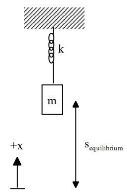
First, let’s place the origin of our coordinate system at the equilibrium location of the bungee jumper. Note, the initial position of the jumper is not the equilibrium position. The equilibrium position is where the net force on the bungee jumper is zero.

To find the equilibrium position:

$$\begin{aligned} &\Sigma F=m a \\ &-F_{\text {gravity }}+F_{\text {spring }}=m a \\ &-m g+k s_{\text {equilibrium }}=m(0) \\ &S_{\text {equilibrium }}=\frac{m g}{k} \end{aligned} \nonumber$$

Now let’s apply Newton’s second law when the jumper is at an arbitrary position, x, with the origin of the coordinate system at the equilibrium position.

$$\begin{aligned} &\Sigma F=m a \\ &-F_{\text {gravity }}+F_{\text {spring }}=m a \\ &-m g+k s=m a \end{aligned} \nonumber$$

Where “s” is the stretch of the spring. The spring is stretched by an amount

$$S=S_{\text {equilibrium }}-x \nonumber$$

Therefore,

$$\begin{aligned} &-m g+k\left(s_{\text {equilibrium }}-x\right)=m a \\ &-m g+k\left(\frac{m g}{k}-x\right)=m a \\ &-m g+m g-k x=m a \\ &-k x=m a \\ &-\frac{k}{m} x=\frac{d^{2} x}{d t^{2}} \end{aligned} \nonumber$$

This is exactly the same differential equation solved earlier. Thus, the motion of the bungee jumper must be described by

$$x(t)=A \cos (\omega t+\phi) \nonumber$$

Now let’s determine the values of $\omega$, A and $\phi$:

From

$$\begin{aligned} &\omega=\sqrt{\frac{k}{m}} \\ &\omega=\sqrt{\frac{35 N / m}{80 k g}} \\ &\omega=0.661 s^{-1} \end{aligned} \nonumber$$

Since A is the maximum displacement of the object from equilibrium,

$$\begin{aligned} &A=S_{\text {equilibrium }} \\ &A=\frac{m g}{k} \\ &A=\frac{80(9.8)}{35} \\ &A=22.4 \mathrm{~m} \end{aligned} \nonumber$$

So now we have

$$x(t)=22.4 \cos (0.661 t+\phi) \nonumber$$

and all that’s left to determine is $\phi$. At t = 0 s, the bungee jumper is at x = 22.4 m. Thus,

$$\begin{aligned} &x(t)=22.4 \cos (0.661 t+\phi) \\ &x(0)=22.4 \cos (0.661(0)+\phi) \\ &22.4=22.4 \cos (\phi) \\ &1=\cos (\phi) \\ &\phi=0 \end{aligned} \nonumber$$

This really shouldn’t surprise you since if you graphed the jumper’s motion it would be a perfect cosine function with no initial phase shift. Thus, the position of the bungee jumper as a function of time is:

$$x(t)=22.4 \cos (0.661 t) \nonumber$$

Since we have the position of the jumper at all times, we can determine everything about the jumper’s motion. For example, her velocity

$$\begin{aligned} &v(t)=\frac{d x(t)}{d t} \\ &v(t)=\frac{d}{d t}(22.4 \cos (0.661 t)) \\ &v(t)=-14.8 \sin (0.661 t) \end{aligned} \nonumber$$

and her maximum speed

$$\left|v_{\max }\right|=14.8 \mathrm{~m} / \mathrm{s} \nonumber$$

which occurs as she passes through the equilibrium position.

Her acceleration

$$\begin{aligned} a(t) &=\frac{d v(t)}{d t} \\ a(t) &=\frac{d}{d t}(-14.8 \sin (0.661 t)) \\ a(t) &=-9.8 \cos (0.661 t) \end{aligned} \nonumber$$

and her maximum acceleration

$$\left|a_{\mathrm{max}}\right|=9.8 \mathrm{~m} / \mathrm{s}^{2} \nonumber$$

which occurs the instant she steps off of the platform (and at the very bottom of her motion).

The time for her to travel through an entire cycle

$$\begin{aligned} T &=\frac{2 \pi}{\omega} \\ T &=\frac{2 \pi}{0.661} \\ T &=9.51 s \end{aligned} \nonumber$$

And on and on and on...

The Physical Pendulum

A 0.4 kg meterstick is hung from a pin attached to one end. The meterstick is displaced by 0.1 radian (5.7⁰) from equilibrium (straight down) and released. After ten complete cycles, the amplitude of the oscillation has decreased to 0.08 radian. Assume a drag force proportional to the speed of the CM of the stick acts at the location of the CM.

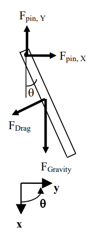
At left is a free-body diagram of the meterstick when it is at an angle $\theta$ from equilibrium, and moving counterclockwise, i.e., swinging up to the right. Since the oscillatory behavior is occurring in the angular direction, let’s write Newton’s second law in angular form:

$$\begin{aligned} &\Sigma \tau=I \alpha \\ &\tau_{\text {drag }}+\tau_{\text {gravity }}=I \alpha \\ &-\frac{L}{2} F_{\text {drag }} \sin 90-\frac{L}{2}(m g) \sin \theta=I \alpha \end{aligned} \nonumber$$

A meterstick can be approximated as a thin rod, and a thin rod rotated about its CM has rotational inertia $\frac{1}{12} \mathrm{~mL}^{2}$. We need the rotational inertia about an axis at one end, so we must use the parallel-axis theorem with $\mathrm{r}_{\mathrm{CM}}=\frac{L}{2}$. Thus,

$$\begin{aligned} &I=m {r_{C M}}^{2}+I_{C M} \\ &I=m\left(\frac{L}{2}\right)^{2}+\frac{1}{12} m L^{2} \\ &I=\frac{1}{4} m L^{2}+\frac{1}{12} m L^{2} \\ &I=\frac{1}{3} m L^{2} \end{aligned} \nonumber$$

So

$$\begin{aligned} &-\frac{L}{2} F_{\text {drag }} \sin 90-\frac{L}{2}(m g) \sin \theta=\left(\frac{1}{3} m L^{2}\right) \alpha \\ &-\frac{1}{2} F_{\text {drag }}-\frac{1}{2} m g \sin \theta=\frac{1}{3} m L \alpha \end{aligned} \nonumber$$

Since the magnitude of the drag force is proportional to the speed of the CM,

$$F_{d r a g}=b v_{C M} \nonumber$$

and⁵

$$\begin{aligned} &v=r \omega \\ &v_{C M}=\frac{L}{2} \omega \end{aligned} \nonumber$$

the drag can be written as

$$F_{\text {drag }}=b\left(\frac{L}{2} \omega\right) \nonumber$$

resulting in:

$$\begin{aligned} &-\frac{1}{2}\left(b\left(\frac{L}{2} \omega\right)\right)-\frac{1}{2} m g \sin \theta=\frac{1}{3} m L \alpha \\ &-\frac{1}{4} b L \omega-\frac{1}{2} m g \sin \theta=\frac{1}{3} m L \alpha \end{aligned} \nonumber$$

Multiplying by 3/L yields:

$$\begin{aligned} &-\frac{3 b}{4} \omega-\frac{3 m g}{2 L} \sin \theta=m \alpha \\ &-\frac{3 m g}{2 L} \sin \theta-\frac{3 b}{4} \frac{d \theta}{d t}=m \frac{d^{2} \theta}{d t^{2}} \end{aligned} \nonumber$$

Since the angle of displacement is small, we will use a common approximation for small angles:

$$\sin \theta \approx \theta \nonumber$$

(For the maximum angle attained by our meterstick, sin (0.1) = 0.998)

Note

⁵ The $\omega$ in the following relationship is the angular velocity of the meterstick (which varies as the meterstick oscillates), not the angular frequency of the meterstick (which is a constant). I know they are the same symbol, but try to keep them straight by examining the context in which they appear.

Using this approximation, our equation becomes:

$$-\frac{3 m g}{2 L} \theta-\frac{3 b}{4} \frac{d \theta}{d t}=m \frac{d^{2} \theta}{d t^{2}} \nonumber$$

This is exactly the same differential equation as the damped linear oscillator,

$$-k x-b \frac{d x}{d t}=m \frac{d^{2} x}{d t^{2}} \nonumber$$

if:

• k is replaced by $\frac{3mg}{2L}$
• b is replaced by $\frac{3b}{4}$
• and the position (x) is replaced by the angular position ($\theta$).

Thus, the effective spring constant is $\frac{3mg}{2 L}$ and the effective damping coefficient is $\frac{3b}{4}$.

Since it is the same differential equation, the motion of the meterstick must be described by the same function:

$$\theta(t)=A e^{-\alpha t} \cos \left(\omega^{\prime} t+\phi\right) \nonumber$$

Now let’s determine the values of A, $\phi$, $\alpha$, and $\omega^{\prime}$:

• Since the meterstick is displaced by 0.1 radian from equilibrium and then released,
  $$\mathrm{A}=0.1 \ \mathrm{rad} \nonumber$$
• Since the maximum displacement of the meterstick occurs at t = 0 s,
  $$\phi=0 \nonumber$$
• In the original differential equation
  $$\alpha=\frac{b}{2 m} \nonumber$$

  Since the effective damping coefficient is $\frac{3b}{4}$,

  $$\begin{aligned} &\alpha=\frac{\left(\frac{3 b}{4}\right)}{2 m} \\ &\alpha=\frac{3 b}{8 m} \\ &\alpha=\frac{3 b}{8(0.4)} \\ &\alpha=0.938 b \end{aligned} \nonumber$$

• In the original differential equation
  $$\omega=\sqrt{\frac{k}{m}} \nonumber$$
  Since the effective spring constant is $\frac{3mg}{2L}$
  $$\begin{aligned} &\omega=\sqrt{\frac{\left(\frac{3 m g}{2 L}\right)}{m}} \\ &\omega=\sqrt{\frac{3 g}{2 L}} \end{aligned} \nonumber$$
  Notice that the angular frequency in the undamped case does not depend on the mass of the meterstick.
  $$\begin{aligned} &\omega=\sqrt{\frac{3\left(9.8 m / s^{2}\right)}{2(1 m)}} \\ &\omega=3.83 s^{-1} \end{aligned} \nonumber$$
  Finally
  $$\begin{aligned} &\omega^{\prime}=\sqrt{\omega^{2}-\alpha^{2}} \\ &\omega^{\prime}=\sqrt{3.83^{2}-(0.938 b)^{2}} \\ &\omega^{\prime}=\sqrt{14.7-0.880 b^{2}} \end{aligned} \nonumber$$

Putting it all together,

$$\theta(t)=0.1 e^{-0.938 b t} \cos \left(\omega^{\prime} t\right) \nonumber$$

with

$$\omega^{\prime}=\sqrt{14.7-0.880 b^{2}} \nonumber$$

Now we can use the information about the effects of damping to determine b. We know that at a time equal to ten periods, the amplitude is 0.08 radians. Since the initial amplitude of the motion was 0.1 radian, the exponential factor, exp(0.938bt) , must be equal to 0.8 when t = 10 T:

$$\begin{aligned} &\exp (-0.938 b(10 T))=0.8 \\ &\exp \left(-9.38 b\left(\frac{2 \pi}{\omega^{\prime}}\right)\right)=0.8 \\ &\exp \left(-58.9 \frac{b}{\omega^{\prime}}\right)=0.8 \\ &-58.9 \frac{b}{\omega^{\prime}}=\ln (0.8) \\ &-58.9 \frac{b}{\omega^{\prime}}=-0.223 \\ &\frac{b}{\omega^{\prime}}=3.79 \times 10^{-3} \\ &b=3.79 \times 10^{-3} \omega^{\prime} \\ &b=3.79 x 10^{-3} \sqrt{14.7-0.880 b^{2}} \\ &b^{2}=1.43 x 10^{-5}\left(14.7-0.880 b^{2}\right) \\ &b^{2}=2.11 x 10^{-4}-1.26 x 10^{-5} b^{2} \\ &b^{2}=2.11 x 10^{-4} \\ &b=0.0145 \mathrm{~kg} / \mathrm{s} \end{aligned} \nonumber$$

Thus,

$$\begin{aligned} &\omega^{\prime}=\sqrt{14.7-0.880 b^{2}} \\ &\omega^{\prime}=\sqrt{14.7-0.000185} \\ &\omega^{\prime}=3.83 s^{-1} \end{aligned} \nonumber$$

Notice that the change in angular frequency due to damping is extremely small. (It is so small that it does not have an effect in the first three significant figures of the angular frequency.)

Finally,

$$\begin{aligned} &\theta(t)=0.1 e^{-0.938(0.0145) t} \cos (3.83 t) \\ &\theta(t)=0.1 e^{-0.0136 t} \cos (3.83 t) \end{aligned} \nonumber$$

This is a complete description of the motion of the meterstick. As in the first example, we can determine anything we desire about the motion of this meterstick through a manipulation of this function.