
3.5: Thermodynamic Processes


- Last updated
- Mar 3, 2025
- Save as PDF

( \newcommand{\kernel}{\mathrm{null}\,}\)
By the end of this section, you will be able to:
- Define a thermodynamic process
- Distinguish between quasi-static and non-quasi-static processes
- Calculate physical quantities, such as the heat transferred, work done, and internal energy change for isothermal, adiabatic, and cyclical thermodynamic processes
In solving mechanics problems, we isolate the body under consideration, analyze the external forces acting on it, and then use Newton’s laws to predict its behavior. In thermodynamics, we take a similar approach. We start by identifying the part of the universe we wish to study; it is also known as our system. (We defined a system at the beginning of this chapter as anything whose properties are of interest to us; it can be a single atom or the entire Earth.) Once our system is selected, we determine how the environment, or surroundings, interact with the system. Finally, with the interaction understood, we study the thermal behavior of the system with the help of the laws of thermodynamics.
The thermal behavior of a system is described in terms of thermodynamic variables. For an ideal gas, these variables are pressure, volume, temperature, and the number of molecules or moles of the gas. Different types of systems are generally characterized by different sets of variables. For example, the thermodynamic variables for a stretched rubber band are tension, length, temperature, and mass.
The state of a system can change as a result of its interaction with the environment. The change in a system can be fast or slow and large or small. The manner in which a state of a system can change from an initial state to a final state is called a thermodynamic process. For analytical purposes in thermodynamics, it is helpful to divide up processes as either quasi-static or non-quasi-static, as we now explain.
Quasi-static and Non-quasi-static Processes
A quasi-static process refers to an idealized or imagined process where the change in state is made infinitesimally slowly so that at each instant, the system can be assumed to be at a thermodynamic equilibrium with itself and with the environment. For instance, imagine heating 1 kg of water from a temperature 20oC to 21oC at a constant pressure of 1 atmosphere. To heat the water very slowly, we may imagine placing the container with water in a large bath that can be slowly heated such that the temperature of the bath can rise infinitesimally slowly from 20oC to 21oC. If we put 1 kg of water at 20oC directly into a bath at 21oC the temperature of the water will rise rapidly to 21oC in a non-quasi-static way.
Quasi-static processes are done slowly enough that the system remains at thermodynamic equilibrium at each instant, despite the fact that the system changes over time. The thermodynamic equilibrium of the system is necessary for the system to have well-defined values of macroscopic properties such as the temperature and the pressure of the system at each instant of the process. Therefore, quasi-static processes can be shown as well-defined paths in state space of the system.
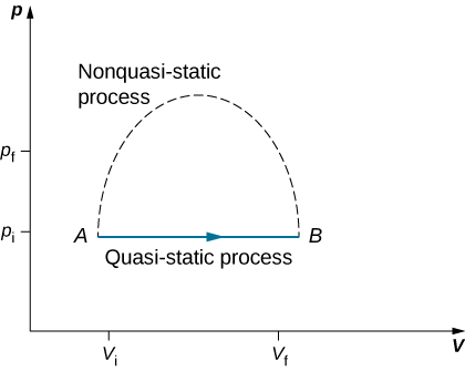
Since quasi-static processes cannot be completely realized for any finite change of the system, all processes in nature are non-quasi-static. Examples of quasi-static and non-quasi-static processes are shown in Figure 3.5.1. Despite the fact that all finite changes must occur essentially non-quasi-statically at some stage of the change, we can imagine performing infinitely many quasi-static process corresponding to every quasi-static process. Since quasi-static processes can be analyzed analytically, we mostly study quasi-static processes in this book. We have already seen that in a quasi-static process the work by a gas is given by pdV.
Isothermal Processes
An isothermal process is a change in the state of the system at a constant temperature. This process is accomplished by keeping the system in thermal equilibrium with a large heat bath during the process. Recall that a heat bath is an idealized “infinitely” large system whose temperature does not change. In practice, the temperature of a finite bath is controlled by either adding or removing a finite amount of energy as the case may be.
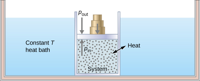
As an illustration of an isothermal process, consider a cylinder of gas with a movable piston immersed in a large water tank whose temperature is maintained constant. Since the piston is freely movable, the pressure inside Pin is balanced by the pressure outside Pout by some weights on the piston, as in Figure 3.5.2.
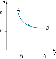
As weights on the piston are removed, an imbalance of forces on the piston develops. The net nonzero force on the piston would cause the piston to accelerate, resulting in an increase in volume. The expansion of the gas cools the gas to a lower temperature, which makes it possible for the heat to enter from the heat bath into the system until the temperature of the gas is reset to the temperature of the heat bath. If weights are removed in infinitesimal steps, the pressure in the system decreases infinitesimally slowly. This way, an isothermal process can be conducted quasi-statically. An isothermal line on a (p, V) diagram is represented by a curved line from starting point A to finishing point B, as seen in Figure 3.5.3. For an ideal gas, an isothermal process is hyperbolic, since for an ideal gas at constant temperature, p∝1V.
An isothermal process studied in this chapter is quasi-statically performed, since to be isothermal throughout the change of volume, you must be able to state the temperature of the system at each step, which is possible only if the system is in thermal equilibrium continuously. The system must go out of equilibrium for the state to change, but for quasi-static processes, we imagine that the process is conducted in infinitesimal steps such that these departures from equilibrium can be made as brief and as small as we like.
Other quasi-static processes of interest for gases are isobaric and isochoric processes. An isobaric process is a process where the pressure of the system does not change, whereas an isochoric process is a process where the volume of the system does not change.
Adiabatic Processes
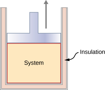
In an adiabatic process, the system is insulated from its environment so that although the state of the system changes, no heat is allowed to enter or leave the system, as seen in Figure 3.5.3. An adiabatic process can be conducted either quasi-statically or non-quasi-statically. When a system expands adiabatically, it must do work against the outside world, and therefore its energy goes down, which is reflected in the lowering of the temperature of the system. An adiabatic expansion leads to a lowering of temperature, and an adiabatic compression leads to an increase of temperature. We discuss adiabatic expansion again in the section on Adiabatic Processes for an ideal Gas.
Cyclic Processes
We say that a system goes through a cyclic process if the state of the system at the end is same as the state at the beginning. Therefore, state properties such as temperature, pressure, volume, and internal energy of the system do not change over a complete cycle: ΔEint=0.
When the first law of thermodynamics is applied to a cyclic process, we obtain a simple relation between heat into the system and the work done by the system over the cycle:
Q=W(cyclicprocess).
Thermodynamic processes are also distinguished by whether or not they are reversible. A reversible process is one that can be made to retrace its path by differential changes in the environment. Such a process must therefore also be quasi-static. Note, however, that a quasi-static process is not necessarily reversible, since there may be dissipative forces involved. For example, if friction occurred between the piston and the walls of the cylinder containing the gas, the energy lost to friction would prevent us from reproducing the original states of the system.
We considered several thermodynamic processes:
- An isothermal process, during which the system’s temperature remains constant
- An adiabatic process, during which no heat is transferred to or from the system
- An isobaric process, during which the system’s pressure does not change
- An isochoric process, during which the system’s volume does not change
Many other processes also occur that do not fit into any of these four categories.
View this site to set up your own process in a pV diagram. See if you can calculate the values predicted by the simulation for heat, work, and change in internal energy.