4.1: Kinetic Energy

For a long time in the development of classical mechanics, physicists were aware of the existence of two different quantities that one could define for an object of inertia \(m\) and velocity \(v\). One was the momentum, \(mv\), and the other was something proportional to \(mv^2\). Despite their obvious similarities, these two quantities exhibited different properties and seemed to be capturing different aspects of motion.

When things got finally sorted out, in the second half of the 19th century, the quantity \(\frac{1}{2}mv^2\) came to be recognized as a form of energy—itself perhaps the most important concept in all of physics. Kinetic energy, as this quantity is called, may be the most obvious and intuitively understandable kind of energy, and so it is a good place to start our study of the subject.

We will use the letter \(K\) to denote kinetic energy, and, since it is a form of energy, we will express it in the units especially named for this purpose, which is to say joules (J). 1 joule is 1 kg·m²/s². In the definition

\[ K=\frac{1}{2} m v^{2} \label{eq:4.1} \]

the letter \(v\) is meant to represent the magnitude of the velocity vector, that is to say, the speed of the particle. Hence, unlike momentum, kinetic energy is not a vector, but a scalar : there is no sense of direction associated with it. In three dimensions, one could write

\[ K=\frac{1}{2} m\left(v_{x}^{2}+v_{y}^{2}+v_{z}^{2}\right) \label{eq:4.2} \]

There is, therefore, some amount of kinetic energy associated with each component of the velocity vector, but in the end they are all added together in a lump sum.

For a system of particles, we will treat kinetic energy as an additive quantity, just like we did for momentum, so the total kinetic energy of a system will just be the sum of the kinetic energies of all the particles making up the system. Note that, unlike momentum, this is a scalar (not a vector) sum, and most importantly, that kinetic energy is, by definition, always positive, so there can be no question of a “cancellation” of one particle’s kinetic energy by another, again unlike what happened with momentum. Two objects of equal mass moving with equal speeds in opposite directions have a total momentum of zero, but their total kinetic energy is definitely nonzero. Basically, the kinetic energy of a system can never be zero as long as there is any kind of motion going on in the system.

Kinetic Energy in Collisions

To gain some further insights into the concept of kinetic energy, and the ways in which it is different from momentum, it is useful to look at it in the same setting in which we “discovered” momentum, namely, one-dimensional collisions in an isolated system. If we look again at the collision represented in Figure 3.1.1 of Chapter 3, reproduced below,

Figure 3.1.1)

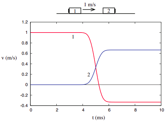
we can use the definition (\ref{eq:4.1}) to calculate the initial and final values of \(K\) for each object, and for the system as a whole. Remember we found that, for this particular system, \(m_2 = 2m_1\), so we can just set \(m_1 \)= 1 kg and \(m_2\) = 2 kg, for simplicity. The initial and final velocities are \(v_{1i}\) = 1 m/s, \(v_{2i}\) = 0, \(v_{1f}\) = −1/3 m/s, \(v_{2f}\) = 2/3 m/s, and so the kinetic energies are

\[ K_{1 i}=\frac{1}{2} \: \mathrm{J}, K_{2 i}=0 ; \quad K_{1 f}=\frac{1}{18} \: \mathrm{J}, K_{2 f}=\frac{4}{9} \: \mathrm{J} \nonumber .\]

Note that 1/18 + 4/9 = 9/18 = 1/2, and so

\[ K_{s y s, i}=K_{1 i}+K_{2 i}=\frac{1}{2} \: \mathrm{J}=K_{1 f}+K_{2 f}=K_{s y s, f} \nonumber .\]

In words, we find that, in this collision, the final value of the total kinetic energy is the same as its initial value, and so it looks like we have “discovered” another conserved quantity (besides momentum) for this system.

This belief may be reinforced if we look next at the collision depicted in Figure 3.1.2 of Chapter 3, again reproduced below. Recall I pointed out back then that we can think of this as being really the same collision as depicted in Figure 3.1.1, only looked at from another frame of reference (one moving initially to the right at 1 m/s). We will have more to say about how to transform quantities from a frame of reference to another by the end of the chapter.

Figure 3.1.2.)

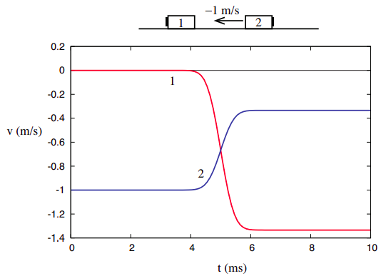
In any case, as observed there, all we need to do is add −1 m/s to all the velocities in the previous problem, so we have \(v_{1i}\) = 0, \(v_{2i}\) = −1 m/s, \(v_{1f}\) = −4/3 m/s, \(v_{2f}\) = −1/3 m/s. The corresponding kinetic energies are, accordingly, \(K_{1i}\) = 0, \(K_{2i}\) = 1 J, \(K_{1f}\) = \(\frac{8}{9}\) J, \(K_{2f}\) = \(\frac{1}{9}\) J. These are all different from the values we had in the previous example, but note that once again the total kinetic energy after the collision equals the total kinetic energy before—namely, 1 J in this case¹ .

Things are, however, very different when we consider the third collision example shown in Chapter 3, namely, the one where the two objects are stuck together after the collision.

Figure 3.1.3)

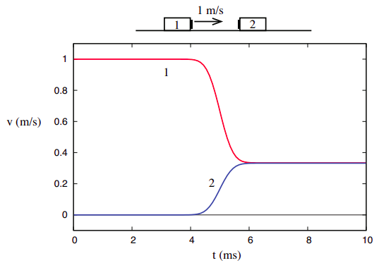
Their joint final velocity, consistent with conservation of momentum, is \(v_{1f}\) = \(v_{2f}\) = 1/3 m/s. Since the system starts as in Figure \(\PageIndex{1}\), its kinetic energy is initially \(K_{sys,i} = \frac{1}{2}\) J, but after the collision we have only

\[ K_{s y s, f}=\frac{1}{2}(3 \: \mathrm{kg})\left(\frac{1}{3} \: \frac{\mathrm{m}}{\mathrm{s}}\right)^{2}=\frac{1}{6} \: \mathrm{J} \nonumber .\]

What this shows, however, is that unlike the total momentum of a system, which is completely unaffected by internal interactions, the total kinetic energy does depend on the details of the interaction, and thus conveys some information about its nature. We can then refine our study of collisions to distinguish two kinds: the ones where the initial kinetic energy is recovered after the collision, which we will call elastic, and the ones where it is not, which we call inelastic. A special case of inelastic collision is the one called totally inelastic, where the two objects end up stuck together, as in Figure \(\PageIndex{3}\). As we shall see later, the kinetic energy “deficit” is largest in that case.

I have said above that in an elastic collision the kinetic energy is “recovered,” and I prefer this terminology to “conserved,” because, in fact, unlike the total momentum, the total kinetic energy of a system does not remain constant throughout the interaction, not even during an elastic collision. The simplest example to show this would be an elastic, head-on collision between two objects of equal mass, moving at the same speed towards each other. In the course of the collision, both objects are brought momentarily to a halt before they reverse direction and bounce back, and at that instant, the total kinetic energy is zero.

You can also examine Figures \(\PageIndex{1}\) and \(\PageIndex{2}\) above, and calculate, from the graphs, the value of the total kinetic energy during the collision. You will see that it dips to a minimum, and then comes back to its initial value (see also Figure \(\PageIndex{4}\), later in this chapter). Conventionally, we may talk of kinetic energy as being “conserved” in elastic collisions, but it is important to realize that we are looking at a different kind of “conservation” than what we had with the total momentum, which was constant before, during, and after the interaction, as long as the system remained isolated.

Elastic collisions do suggest that, whatever the ultimate nature of this thing we call “energy” might be, it may be possible to store it in some form (in this case, during the course of the collision), and then recover it, as kinetic energy, eventually. This paves the way for the introduction of other kinds of “energy” besides kinetic energy, as we shall see in a later chapter, and the possibility of interconversion to take place among these kinds. For the moment, we shall simply say that in an elastic collision some amount of kinetic energy is temporarily stored as some kind of “internal energy,” and after the collision this is converted back into kinetic energy; whereas, in an inelastic collision, some amount of kinetic energy gets irrevocably converted into some “internal energy,” and we never get it back.

Since whatever ultimately happens depends on the details and the nature of the interaction, we will be led to distinguish between “conservative” interactions, where kinetic energy is reversibly stored as some other form of energy somewhere, and “dissipative” interactions, where the energy conversion is, at least in part, irreversible. Clearly, elastic collisions are associated with conservative interactions and inelastic collisions are associated with dissipative interactions. This preliminary classification of interactions will have to be reviewed a little more carefully, however, in the next chapter.

---

¹This is, of course, consistent with the principle of relativity I told you about in Chapter 2: if the process in Figure \(\PageIndex{2}\) is really the same as the one in Figure \(\PageIndex{1}\), only viewed in a different inertial reference frame, then, if energy is seen to be conserved in one frame, it should also be seen to be conserved in the other. More on this in Section 4.2.

---

Relative Velocity and Coefficient of Restitution

An interesting property of elastic collisions can be disclosed from a careful study of figures \(\PageIndex{1}\) and \(\PageIndex{2}\). In both cases, as you can see, the relative velocity of the two objects colliding has the same magnitude (but opposite sign) before and after the collision. In other words: in an elastic collision, the objects end up moving apart at the same rate as they originally came together.

Recall that, in Chapter 1, we defined the velocity of object 2 relative to object 1 as the quantity

\[ v_{12}=v_{2}-v_{1} \label{eq:4.3} \]

(compare Equation (1.3.8); and similarly the velocity of object 1 relative to object 2 is \(v_{21} = v_1 − v_2\). With this definition you can check that, indeed, the collisions shown in Figs. \(\PageIndex{1}\) and \(\PageIndex{2}\) satisfy the equality

\[ v_{12, i}=-v_{12, f} \label{eq:4.4} \]

(note that we could equally well have used \(v_{21}\) instead of \(v_{12}\)). For instance, in Figure \(\PageIndex{1}\), \(v_{12,i} = v_{2i} − v_{1i}\) = −1 m/s, whereas \(v_{12,f}\) = 2/3 − (−1/3) = 1 m/s. So the objects are initially moving towards each other at a rate of 1 m per second, and they end up moving apart just as fast, at 1 m per second. Visually, you should notice that the distance between the red and blue curves is the same before and after (but not during) the collision; the fact that they cross accounts for the difference in sign of the relative velocity, which in turns means simply that before the collision they were coming together, and afterwards they are moving apart.

It takes only a little algebra to show that Equation (\ref{eq:4.4}) follows from the joint conditions of conservation of momentum and conservation of kinetic energy. The first one (\(p_i\) = \(p_f\) ) clearly has the form

\[ m_{1} v_{1 i}+m_{2} v_{2 i}=m_{1} v_{1 f}+m_{2} v_{2 f} \label{eq:4.5} \]

whereas the second one (\(K_i\) = \(K_f\) ) can be written as

\[ \frac{1}{2} m_{1} v_{1 i}^{2}+\frac{1}{2} m_{2} v_{2 i}^{2}=\frac{1}{2} m_{1} v_{1 f}^{2}+\frac{1}{2} m_{2} v_{2 f}^{2} \label{eq:4.6} .\]

We can cancel out all the factors of 1/2 in Equation (\ref{eq:4.6})², then rearrange it so that quantities belonging to object 1 are on one side, and quantities belonging to object 2 are on the other. We get

\begin{array}{c}
{m_{1}\left(v_{1 i}^{2}-v_{1 f}^{2}\right)=-m_{2}\left(v_{2 i}^{2}-v_{2 f}^{2}\right)} \\
{m_{1}\left(v_{1 i}-v_{1 f}\right)\left(v_{1 i}+v_{1 f}\right)=-m_{2}\left(v_{2 i}-v_{2 f}\right)\left(v_{2 i}+v_{2 f}\right)} \label{eq:4.7}
\end{array}

(using the fact that \(a^2 − b^2 = (a + b)(a − b) \)). Note, however, that Equation (\ref{eq:4.5}) can also be rewritten as

\[ m_{1}\left(v_{1 i}-v_{1 f}\right)=-m_{2}\left(v_{2 i}-v_{2 f}\right) \nonumber .\]

This immediately allows us to cancel out the corresponding factors in Eq (\ref{eq:4.7}), so we are left with \(v_{1i} + v_{1f} = v_{2i} + v_{2f} \), which can be rewritten as

\[ v_{1 f}-v_{2 f}=v_{2 i}-v_{1 i} \label{eq:4.8} \]

and this is equivalent to (\ref{eq:4.4})

So, in an elastic collision the speed at which the two objects move apart is the same as the speed at which they came together, whereas, in what is clearly the opposite extreme, in a totally inelastic collision the final relative speed is zero—the objects do not move apart at all after they collide. This suggests that we can quantify how inelastic a collision is by the ratio of the final to the initial magnitude of the relative velocity. This ratio is denoted by \(e\) and is called the coefficient of restitution. Formally,

\[ e=-\frac{v_{12, f}}{v_{12, i}}=-\frac{v_{2 f}-v_{1 f}}{v_{2 i}-v_{1 i}} \label{eq:4.9} .\]

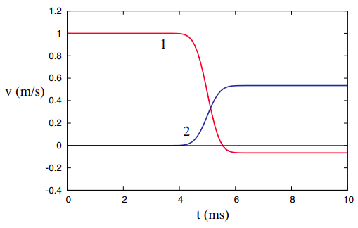
For an elastic collision, \(e\) = 1, as required by Equation (\ref{eq:4.4}). For a totally inelastic collision, like the one depicted in Figure \(\PageIndex{3}\), \(e\) = 0. For a collision that is inelastic, but not totally inelastic, \(e\) will have some value in between these two extremes. This knowledge can be used to “design” inelastic collisions (for homework problems, for instance!): just pick a value for \(e\), between 0 and 1, in Equation (\ref{eq:4.9}), and combine this equation with the conservation of momentum requirement (\ref{eq:4.5}). The two equations then allow you to calculate the final velocities for any values of \(m_1\), \(m_2\), and the initial velocities. Figure \(\PageIndex{4}\) below, for example, shows what the collision in Figure \(\PageIndex{1}\) would have been like, if the coefficient of restitution had been 0.6 instead of 1. You can check, by solving (\ref{eq:4.5}) and (\ref{eq:4.9}) together, and using the initial velocities, that \(v_{1f}\) = −1/15 m/s = −0.0667 m/s, and \(v_{2f}\) = 8/15 m/s = 0.533 m/s.

Figure \(\PageIndex{1}\).

Although, as I just mentioned, for most “normal” collisions the coefficient of restitution will be a positive number between 1 and 0, there can be exceptions to this. If one of the objects passes through the other (like a bullet through a target, for instance), the value of \(e\) will be negative (although still between 0 and 1 in magnitude). And \(e\) can be greater than 1 for so-called “explosive collisions,” where some amount of extra energy is released, and converted into kinetic energy, as the objects collide. (For instance, two hockey players colliding on the rink and pushing each other away.) In this case, the objects may well fly apart faster than they came together.

An extreme example of a situation with \(e\) > 0 is an explosive separation, which is when the two objects are initially moving together and then fly apart. In that case, the denominator of Equation (\ref{eq:4.9}) is zero, and so \(e\) is formally infinite. This suggests, what is in fact the case, namely, that although explosive processes are certainly important, describing them through the coefficient of restitution is rare, even when it would be formally possible. In practice, use of the coefficient of restitution is mostly limited to the elastic-to-completely inelastic range, that is, 0 ≤ \(e\) ≤ 1.

---

²You may be wondering, just why do we define kinetic energy with a factor 1/2 in front, anyway? There is no good answer at this point. Let’s just say it will make the definition of “potential energy” simpler later, particularly as regards its relationship to force.